Throughout 64 English authorities and 6 2026 situations, even the strongest situation shock was solely 13% of the median uncertainty band.
In plain English: the mannequin’s assumptions moved the end result lower than historic forecast error did. Essentially the most aggressive challenger surge I may parameterise sits contained in the noise the mannequin has produced in previous elections. That’s not a defect. It’s the end result.
I constructed this situation mannequin anticipating clear separation between assumptions. I anticipated S3, the challenger surge, to dominate. I anticipated rankings I may defend. What I received was an envelope the place the strongest shock sits inside calibrated uncertainty, and the place rankings dissolve when intervals are plotted on prime of them.
That is the second instalment of a venture on English native electoral knowledge. Half 1 corrected a categorical-normalisation bug that reversed the unique headline. Half 2 picks up the place the corrected baseline ends and asks a distinct query: given the historic churn we now measure accurately, what 2026 situations are value modelling, and the way ought to we learn them when uncertainty is wider than the shocks?
What was modelled
The 2026 English native elections are scheduled for Thursday 7 Might 2026. This venture covers 64 lively authorities holding elections that day: 32 London boroughs, 27 metropolitan boroughs, and 5 West Yorkshire authorities. Six situations apply totally different assumptions to the identical historic baseline. 4 metrics are computed for every situation × authority mixture: volatility_score, delta_fi, swing_concentration, and turnout_delta. The mannequin produces 1,536 output rows, every with some extent estimate plus calibrated P10, P50, and P90 values from 2,000 attracts of the empirical error distribution.
| State of affairs | Query | Important assumption |
|---|---|---|
| S0 | What if no new swing is utilized? | Historic uncertainty solely |
| S1 | What if 2018-2022 challenger patterns proceed? | Continuation of latest challenger churn |
| S2 | What if main events partially get well? | Institution recovers half misplaced share |
| S3 | What if challengers surge tougher? | Stress take a look at: +4pp challenger surge |
| S4 | What if deprivation-linked turnout rises? | +3pp turnout in IMD deciles 1-3 |
| S5 | What if London volatility is capped by historical past? | London P90 upper-tail cap |
Every situation is a managed perturbation. Labels describe assumptions, not outcomes. The complete interactive dashboard is on Tableau Public.
Two definitions to hold via the remainder of the article: situation shock is the motion within the situation level estimate relative to the baseline. Uncertainty width is the P10-to-P90 interval calibrated from historic forecast error. The 13% headline is the primary divided by the second.
Methodology: backtest errors because the empirical uncertainty distribution
Backtest errors should not only a scorecard. They will change into the empirical uncertainty distribution for future situation evaluation.
The usual use of a backtest is cross/fail. Did the predictions match held-out actuality? That solutions whether or not the mannequin labored, but it surely leaves the residuals on the ground.
A second use treats these residuals as a distribution. How unsuitable has the mannequin been throughout boroughs and cycles, in what path, with what unfold? The reply turns into the empirical pattern from which future uncertainty bands are drawn. Predictive bands cease being parametric assumptions about how errors ought to behave. They’re bootstrapped from how errors even have behaved.
This mannequin makes use of backtests within the second sense. Tier-level mean-centered historic error swimming pools from the 2014→2018 coaching window and the 2018→2022 backtest type the bootstrap pool from which 2026 uncertainty bands are sampled. In sensible phrases: the mannequin is asking how a lot motion would rely as genuinely uncommon relative to the noise it has produced earlier than.
Two design selections form the calibration.
Errors are pooled on the tier stage, not on the borough stage. Every borough has 1-2 prior observations, which is just too noisy to characterise a residual distribution. Pooling on the tier stage (London, Metropolitan, West Yorkshire) retains a pattern massive sufficient to be informative whereas preserving the structural distinction between geographies which have traditionally behaved in another way.
Errors are mean-centered earlier than sampling. This separates historic bias from uncertainty dispersion. With out centering, S0’s P50 would drift away from zero due to historic imply error, mixing the mannequin’s observe document of being barely off into the median of the band. After centering, the band represents dispersion across the situation assumption slightly than dispersion across the mannequin’s bias.
One nuance value flagging: mean-centering removes common historic bias however doesn’t power the bootstrap median to equal the purpose estimate. When residual swimming pools are skewed or bounded (swing_concentration has a decrease sure of 1.0), the P50 can nonetheless sit barely off the belief. Reporting P10/P50/P90 individually, slightly than imply ± commonplace deviation, retains that asymmetry seen.
The two,000 attracts produce steady percentile estimates whereas conserving the complete output below 10,000 rows for clear Tableau ingestion.
Knowledge science takeaway: Backtest errors should not only a scorecard. They will change into the empirical uncertainty distribution for future situation evaluation, calibrating bands that replicate how the mannequin has truly been unsuitable.
The end result: shocks smaller than uncertainty
Three numbers carry the discovering:
- S3 challenger surge: 13% of the median volatility interval.
- S1 volatility continuation: 6%.
- S2 institution restoration: 5%.
Every quantity is the situation shock divided by the median P10-to-P90 band width throughout the 64 lively authorities. The strongest shock, a +4pp challenger surge, strikes the central estimate by about one-eighth of the historic noise the mannequin has produced in previous cycles.
The end result I least anticipated is crucial one: the situations are much less separated than the uncertainty bands. If this had been a forecast dashboard, that may be disappointing. For a situation evaluation, it’s the level.

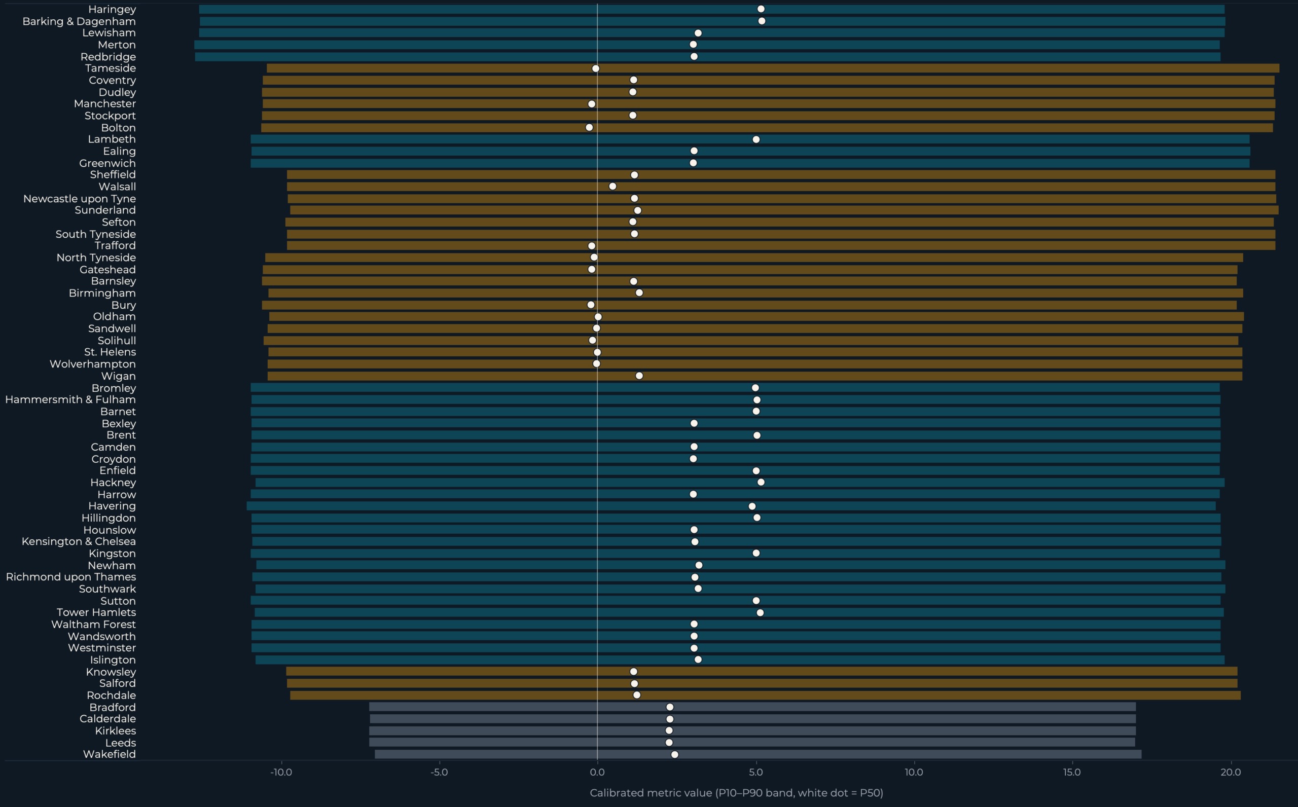
The best way to learn the chart: every horizontal bar is one authority’s calibrated uncertainty interval. The white dot inside it’s the calibrated median. The bar’s color is geographic, not analytical (teal = London, amber = Metropolitan, slate = West Yorkshire). The amber rings exhibiting every situation’s level estimate are seen on the rankings panel (Determine 2b); in Determine 1 they’re summarised within the inset percentages.
Throughout 64 authorities and the three lively situations, the purpose estimate practically at all times sits contained in the bar. The shock perturbs the mannequin lower than the mannequin has traditionally perturbed itself.
Half 1 reported that the correlation between turnout change and volatility was statistically null (r = -0.12, p = 0.35). Half 2 finds that situation shocks are equally smaller than the uncertainty round them. The sample is identical: when the magnitude of an impact is similar to or smaller than the noise, rating the results creates false precision. Impact-vs-uncertainty determines whether or not a end result must be interpreted as sign or context.
The dashboard doesn’t say “S3 wins.” It says S3 strikes the envelope most whereas nonetheless sitting inside broad empirical uncertainty. “Wins” implies the mannequin has chosen between situations. It has not. One situation perturbs the central estimate barely greater than the others; the band round all three stays broad sufficient to soak up the distinction.
Knowledge science takeaway: At all times examine impact measurement to uncertainty width. A situation shock that appears massive in isolation could also be small relative to historic error.
Studying the dashboard: geography and rankings
Two views translate the headline into geographic and ranked context.
The map reveals uncertainty footprint for one situation at a time. Color encodes P50 below the chosen situation; measurement encodes interval width. The widest bands should not solely in London. Metropolitan boroughs within the North East, North West, and West Yorkshire present interval widths similar to the densest London cluster.

The rankings view is the place the effect-vs-uncertainty comparability turns into hardest to disregard. Every row reveals three marks: the bar (P10-P90), the white dot (P50), and the amber ring (situation level estimate). The amber ring practically at all times sits contained in the bar, which implies the situation shock is smaller than the historic uncertainty even for the authorities ranked on the prime.

Rankings of unsure estimates want their intervals proven alongside them. A ranked listing with out uncertainty invitations false precision: the reader sees Authority A above Authority B and assumes the mannequin is assured concerning the order. When the bands overlap, as they do at each stage of those rankings, that confidence is unwarranted.
Two uneven situations, two design classes
Two of the six situations behave in another way from the remaining. S4 and S5 don’t run on the identical vote-share-perturbation logic as S1, S2, and S3, and the distinction makes them helpful design demonstrations past the election context.
S4 lesson: isolate one mechanism at a time.
S4 assessments a speculation from UK turnout literature: that elections in additional disadvantaged authorities can present turnout shifts when native salience modifications. It applies a +3 proportion level turnout shock to authorities falling in IMD deciles 1-3 below the LAD-level Index of A number of Deprivation (IMD 2019) overlay. 41 of the 64 lively authorities obtain the shock; 23 don’t. The tier cut up: 13 of 32 London boroughs, 23 of 27 metropolitan boroughs, all 5 West Yorkshire authorities. Inside this situation scope, the shock concentrates amongst Metropolitan and West Yorkshire authorities greater than amongst London boroughs.

Vote-share metrics (fragmentation, volatility, swing focus) are copied from S0 unchanged below S4. The situation is turnout-only by development.
That development is the design lesson. By conserving S4 to a single perturbation channel, the belief is falsifiable by itself phrases. If noticed 2026 turnout shifts in IMD-1-to-3 authorities should not within the +3pp vary, the belief fails with out dragging the vote-share story with it. A situation that perturbs three mechanisms concurrently is tougher to be taught from when actuality disagrees with it. You can’t inform which assumption broke.
S5 lesson: log guardrails even when they don’t bind.
S5 caps the higher tail of London volatility_score at 39.45. The cap is the empirical ninetieth percentile of historic London borough volatility throughout the coaching and backtest home windows: 64 London borough observations (32 from coaching, 32 from backtest, Metropolis of London excluded as a result of it sits outdoors the 32-borough London electoral scope). The cap is one-sided, applies solely to London, and constrains the P90 solely.
Within the frozen run, the utmost London S5 P90 is 16.70. That’s 42% of the cap, with 22.75 items of headroom. The cap binds zero occasions.
S5 is a guardrail, not an adjustment. It will have constrained the higher tail of London volatility if any borough had exceeded historic ranges. None did. The worth lies in being logged. A stress take a look at that doesn’t bind continues to be helpful provenance: it reveals the analyst thought of the failure mode, parameterised the constraint from knowledge, and reported that the constraint was inactive. Eradicating the cap from the documentation as a result of it didn’t fireplace would erase the analytical determination that was made.
Reproducibility and limitations
The mannequin is frozen, seeded, hashed, and reproducible from the repository. Re-running src/civic_lens/scenario_model.py towards the locked commit reproduces the output bit-for-bit.

One recognized limitation is documented on the dashboard alongside the end result. The coaching window predates Reform UK’s 2025-2026 growth, so right-wing challenger volatility could also be understated below a speculation the place Reform behaves in another way from prior rebel events at scale.
All underlying knowledge is brazenly licensed: election outcomes from the DCLEAPIL v1.0 dataset (Leman 2025, CC BY-SA 4.0); turnout and 2022 cross-checks from the Commons Library native elections dataset (Open Parliament Licence v3.0); deprivation and geography from ONS / MHCLG (OGL v3). The pipeline code within the Civic Lens repository is MIT-licensed; derived knowledge are revealed with supply attribution and stay topic to upstream licences.
Knowledge science takeaway: A mannequin is extra reliable when its outputs are frozen, hashed, and reproducible. Provenance is a part of the evaluation. Limitations must be seen on the identical display screen because the headline quantity.
What situation evaluation teaches us
The transferable ability just isn’t election modelling. It’s constructing situation programs the place assumptions are seen, uncertainty is calibrated towards historic error, and impact sizes are reported alongside the noise that surrounds them. The identical sample reveals up in demand forecasts below price-change situations, public well being coverage stress assessments, and threat fashions the place regulator-imposed shocks are smaller than realised market volatility. Rank situations with out exhibiting the uncertainty round them and also you produce false precision. That’s the lure.
The mannequin doesn’t say what’s going to occur in Might 2026. It says what can be shocking relative to calibrated uncertainty. Three issues to observe on outcomes evening and the times after:
- Whether or not challenger surges exceed the S3 envelope. If realised volatility in challenger-active boroughs exceeds the S3 P90 bands proven on the dashboard, the calibrated band has been breached and the mannequin wants retraining. That is the more than likely place for the mannequin to interrupt, as a result of Reform UK’s post-2024 trajectory is unprecedented within the coaching window.
- Whether or not London volatility breaches the historic upper-tail cap. The S5 cap of 39.45 is the empirical ninetieth percentile throughout 64 historic London observations. A single 2026 borough exceeding it will clear the historic upper-tail threshold. Two or extra can be a significant break with the historic distribution.
- Whether or not deprivation-linked turnout shifts materialise within the path S4 assumes. A clear take a look at of 1 remoted mechanism, with vote-share metrics held fixed. If turnout in IMD-1-to-3 authorities doesn’t transfer within the +3pp vary, the S4 speculation fails by itself phrases.
What occurs after Might 7
The mannequin is already frozen. The hashes, RNG seed, and code commit proven on the provenance dashboard can’t change between now and election evening. Regardless of the calibrated bands say at the moment is what they may say when realised outcomes land.
Half 3 of this sequence might be a public accuracy audit. Frozen situation outputs might be examined towards precise 2026 borough-level outcomes. Protection charges (did P10-P90 include the realised worth?), imply absolute error, rating high quality, and any systematic misses will all be reported, together with the failures. The methodology caveat about Reform UK is the more than likely failure mode; we’ll see whether or not the bands held.
That’s what the freeze permits. The “three issues to observe” above should not rhetorical. They’re the falsification standards for an uncertainty mannequin revealed earlier than its knowledge existed.
Essentially the most sincere end result just isn’t a prediction. It’s a warning about precision. The situations transfer the envelope, however historic uncertainty continues to be wider than the shocks.
For knowledge scientists, which may be the primary lesson: situation evaluation is most helpful when it resists turning into a forecast.
The complete interactive dashboard is revealed on Tableau Public. The pipeline, situation mannequin code, calculated fields, and Tableau construct information are open-source at github.com/Wisabi-Analytics/civic-lens.
Obinna Iheanachor is a Senior AI/Knowledge Engineer and founding father of Wisabi Analytics, a UK-based knowledge engineering and AI consultancy. He creates content material round manufacturing AI programs, knowledge pipelines, and utilized analytics at @DataSenseiObi on X and Wisabi Analytics on YouTube. Civic Lens is an open-source political knowledge venture at github.com/Wisabi-Analytics/civic-lens.


