
On this article, you’ll learn to assume by way of vectorized operations utilizing NumPy, changing sluggish Python loops with environment friendly array-level computations.
Subjects we are going to cowl embody:
- Why Python loops are sluggish for numeric information and the way NumPy’s C-backed engine addresses this.
- Learn how to apply element-wise operations, boolean masking, and broadcasting to remove frequent loop patterns.
- Learn how to deal with multi-condition branching and axis-based aggregation completely with NumPy features.
Introduction
You already know find out how to loop in Python. Loops are easy, readable, they usually do precisely what they are saying. The issue is that at scale, Python loops turn out to be too sluggish. In some unspecified time in the future, each developer working with numeric information begins searching for a greater method.
NumPy’s vectorized operations present that different. As an alternative of telling Python what to do ingredient by ingredient, you describe the transformation on the array degree and let NumPy’s C-backed engine apply it throughout all parts effectively.
This text teaches vectorized pondering by a set of examples. You’ll see the loop-based model, its vectorized equal, and the reasoning behind translating one into the opposite.
You could find the entire code for these examples on GitHub.
Understanding Why Loops Are Gradual In Python
It helps to start out by understanding why the loop you’re changing is sluggish.
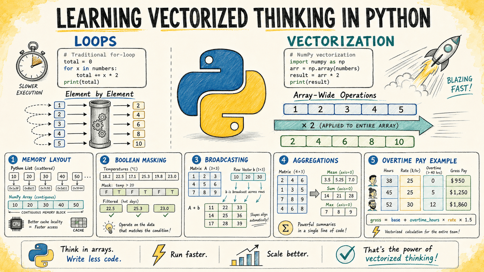
Python is dynamically typed. Each time you write an operation like x * 2 inside a loop, Python should decide the kind of x, discover the right multiplication technique, execute it, and create a brand new Python object for the outcome.
That overhead is insignificant when working with a small variety of parts. However when the identical operation runs throughout tens of millions of values, these repeated Python-level operations add up rapidly.
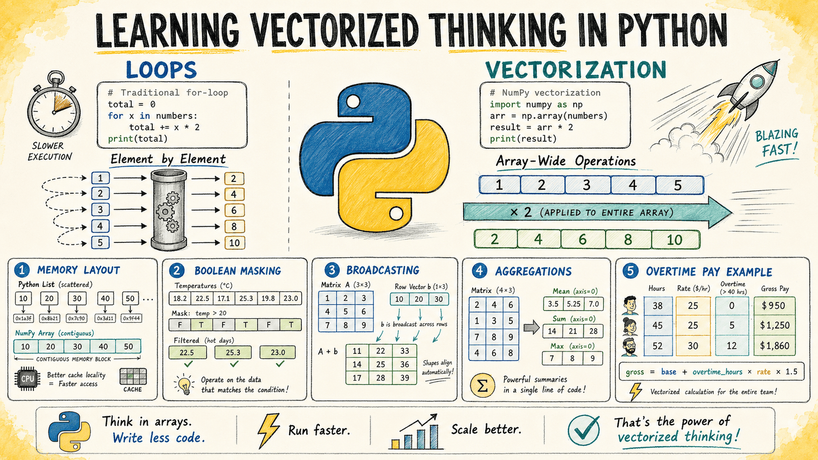
NumPy arrays work in another way. They retailer parts as uncooked numbers in a contiguous block of reminiscence, much like how arrays are saved in C. While you write arr * 2, NumPy passes the complete array to a compiled C routine that applies the operation with out Python overhead for every particular person merchandise.
The computation runs nearer to compiled code pace quite than interpreted Python pace.
Making use of Operations Ingredient By Ingredient
A standard first step with numeric information is making use of the identical formulation to each worth in a listing.
Take into account a easy instance: you could have a listing of product costs and wish to use a 12% tax charge to every merchandise.
Loop Model
The normal method iterates by every value, calculates the taxed worth, and appends the outcome to a brand new checklist.
|
costs = [12.99, 45.00, 7.49, 129.99, 3.25, 89.50]
taxed = [] for value in costs: taxed.append(spherical(value * 1.12, 2))
print(taxed) |
Output:
|
[14.55, 50.4, 8.39, 145.59, 3.64, 100.24] |
Vectorized Model
The vectorized method replaces the loop with a single operation on a NumPy array. While you write costs * 1.12, NumPy applies the multiplication to each ingredient robotically.
|
import numpy as np
costs = np.array([12.99, 45.00, 7.49, 129.99, 3.25, 89.50]) taxed = np.spherical(costs * 1.12, 2)
print(taxed) |
Output:
|
[ 14.55 50.4 8.39 145.59 3.64 100.24] |
The output is an identical, however the method scales a lot better. For big arrays containing tens of millions of costs, the vectorized model might be dramatically quicker than the loop-based equal.
The vital psychological shift is shifting from:
“For every value, carry out this calculation.”
to:
“Apply this transformation to the complete array of costs.”
The array turns into the unit of computation quite than the person ingredient.
Utilizing Boolean Masking For Conditional Logic
Loops usually comprise if statements that test every worth individually. The vectorized equal is a boolean masks: an array of True and False values generated from a comparability.
A boolean masks can then be used to filter values or replace chosen parts with out writing a loop.
Take into account a climate monitoring system that data hourly temperatures. You wish to flag each studying above 38°C as a warmth alert.
Loop Model
The loop method checks every temperature worth and builds a separate checklist of alert flags.
|
readings = [34.1, 38.5, 37.2, 39.0, 36.8, 40.1, 35.5]
alerts = [] for temp in readings: alerts.append(temp > 38.0)
print(alerts) |
Output:
|
[False, True, False, True, False, True, False] |
Vectorized Model
With NumPy, evaluating an array instantly creates the boolean masks robotically. There is no such thing as a express loop and no repeated append() operation.
|
import numpy as np
readings = np.array([34.1, 38.5, 37.2, 39.0, 36.8, 40.1, 35.5])
alerts = readings > 38.0
print(alerts) print(“Alert readings:”, readings[alerts]) |
Output:
|
[False True False True False True False] Alert readings: [38.5 39. 40.1] |
The masks can instantly index again into the unique array and return solely the values that matched the situation.
This sample is among the most vital concepts in vectorized programming:
Compute a masks, then use that masks to pick out or modify values.
It replaces lots of the conditional checks you’ll usually write inside a loop.
For conditional task, np.the place() offers a compact different. For instance, the next operation units excessive temperatures to 38.0 whereas leaving different values unchanged:
|
np.the place(readings > 38.0, 38.0, readings) |
Broadcasting Throughout Totally different Array Shapes
Broadcasting is NumPy’s mechanism for making use of operations between arrays with completely different shapes with out creating pointless copies.
It may possibly really feel extra summary at first, nevertheless it removes many nested loops that might in any other case be wanted to align information buildings manually.
Take into account a sensible instance. Think about you could have click-through charge information for 5 advertising campaigns throughout three channels: e-mail, social, and search. You wish to normalize every channel by dividing values by the utmost worth in that column.
Loop Model
The loop-based method processes every column individually.
|
1 2 3 4 5 6 7 8 9 10 11 12 13 14 15 16 17 18 19 |
import numpy as np
# rows = campaigns, columns = channels (e-mail, social, search) ctr = np.array([ [0.042, 0.031, 0.078], [0.019, 0.055, 0.091], [0.033, 0.047, 0.063], [0.061, 0.028, 0.085], [0.025, 0.039, 0.070], ])
# Loop model: normalize every column individually normalized_loop = np.zeros_like(ctr)
for col in vary(ctr.form[1]): col_max = ctr[:, col].max() normalized_loop[:, col] = ctr[:, col] / col_max
print(normalized_loop) |
Output:
|
[[0.68852459 0.56363636 0.85714286] [0.31147541 1. 1. ] [0.54098361 0.85454545 0.69230769] [1. 0.50909091 0.93406593] [0.40983607 0.70909091 0.76923077]] |
The result’s appropriate, however the logic requires iterating over the columns.
Vectorized Model
The broadcasting method calculates the column maximums as a one-dimensional array and divides the complete matrix in a single operation.
|
col_maxima = ctr.max(axis=0)
normalized = ctr / col_maxima
print(normalized) |
Output:
|
[[0.68852459 0.56363636 0.85714286] [0.31147541 1. 1. ] [0.54098361 0.85454545 0.69230769] [1. 0.50909091 0.93406593] [0.40983607 0.70909091 0.76923077]] |
NumPy sees a (5, 3) array divided by a (3,) array and robotically aligns the shapes. The one-dimensional array is handled conceptually as a row vector and utilized throughout all 5 rows.
No precise copy is created. NumPy handles the operation effectively inside its compiled layer.
The final rule is easy: when a loop exists solely to make array shapes line up, broadcasting is commonly the cleaner answer.
Aggregating Information Alongside An Axis
Many information duties contain summarizing rows or columns of a matrix. NumPy’s discount features, similar to sum(), imply(), max(), and std(), embody an axis argument that determines the course of the discount.
The axis parameter tells NumPy which dimension to break down:
axis=0collapses rows, returning one worth per column.axis=1collapses columns, returning one worth per row.- Leaving
axisunspecified reduces the complete array to a single worth.
Persevering with with the click-through charge information from the earlier instance, you’ll be able to calculate common efficiency per channel and per marketing campaign with out writing any loops.
|
channel_avg = ctr.imply(axis=0) campaign_avg = ctr.imply(axis=1)
print(“Channel averages:”, np.spherical(channel_avg, 4)) print(“Marketing campaign averages:”, np.spherical(campaign_avg, 4)) |
Output:
|
Channel averages: [0.036 0.04 0.0774] Marketing campaign averages: [0.0503 0.055 0.0477 0.058 0.0447] |
The output offers each summaries in solely two traces. A loop-based method would require separate iterations for calculating row and column averages.
With NumPy, the axis argument instantly expresses the intent of the operation.
Changing Multi-Situation Loops
Information processing usually combines a number of circumstances with calculations. Vectorization turns into particularly invaluable when a loop comprises branching logic that handles completely different instances.
Take into account a payroll instance. You’ve got worker hours and hourly charges, and it’s worthwhile to calculate gross pay the place hours above 40 obtain additional time pay at 1.5 occasions the common charge.
Loop Model
The loop model checks every worker individually and applies the right calculation.
|
hours = np.array([38, 45, 40, 52, 33, 41]) charge = np.array([22.50, 18.00, 31.00, 15.50, 27.00, 19.75])
pay_loop = []
for h, r in zip(hours, charge): if h <= 40: pay_loop.append(h * r) else: common = 40 * r additional time = (h – 40) * r * 1.5 pay_loop.append(common + additional time)
print([round(p, 2) for p in pay_loop]) |
Output:
|
[np.float64(855.0), np.float64(855.0), np.float64(1240.0), np.float64(899.0), np.float64(891.0), np.float64(819.62)] |
Vectorized Model
The vectorized method separates the calculation into array operations. Common pay applies to the primary 40 hours, whereas additional time pay applies solely to hours above that threshold.
|
regular_pay = np.minimal(hours, 40) * charge
overtime_pay = np.most(hours – 40, 0) * charge * 1.5
gross_pay = np.spherical(regular_pay + overtime_pay, 2)
print(gross_pay) |
Output:
|
[ 855. 855. 1240. 853.25 891. 839.38] |
The np.minimal() perform caps every worth at 40, robotically dealing with workers who didn’t work additional time.
The np.most() perform calculates additional time hours by subtracting 40 and changing unfavorable values with zero, guaranteeing workers with out additional time contribute nothing to the additional time calculation.
The important thing psychological shift is changing if/else branches with element-wise operations that produce the right outcome for each worth concurrently.
Constructing The Behavior Of Vectorized Considering
Vectorized pondering is a ability that develops with apply. The primary problem is altering your method from describing how Python ought to iterate to describing what the array ought to turn out to be.
While you see a loop that processes numeric information, use this guidelines:
- Does the operation apply the identical formulation to each ingredient? Use array arithmetic.
- Does it filter values based mostly on a situation? Use a boolean masks.
- Does it summarize rows or columns? Use
np.sum(),np.imply(), or comparable features with anaxisargument. - Does it function on arrays with completely different shapes? Verify whether or not broadcasting can exchange the loop.
You shouldn’t, nevertheless, remove each loop in your code. Some issues are naturally iterative, and forcing vectorization could make code more durable to know. Your aim ought to be to acknowledge when the array itself can characterize the complete computation.
From right here, the subsequent step is exploring np.vectorize() for features that don’t map naturally to built-in array operations.
It’s also possible to be taught to vectorize operations in pandas, which builds a column-oriented information construction on high of NumPy arrays and extends the identical vectorized mannequin to labeled, mixed-type datasets.