
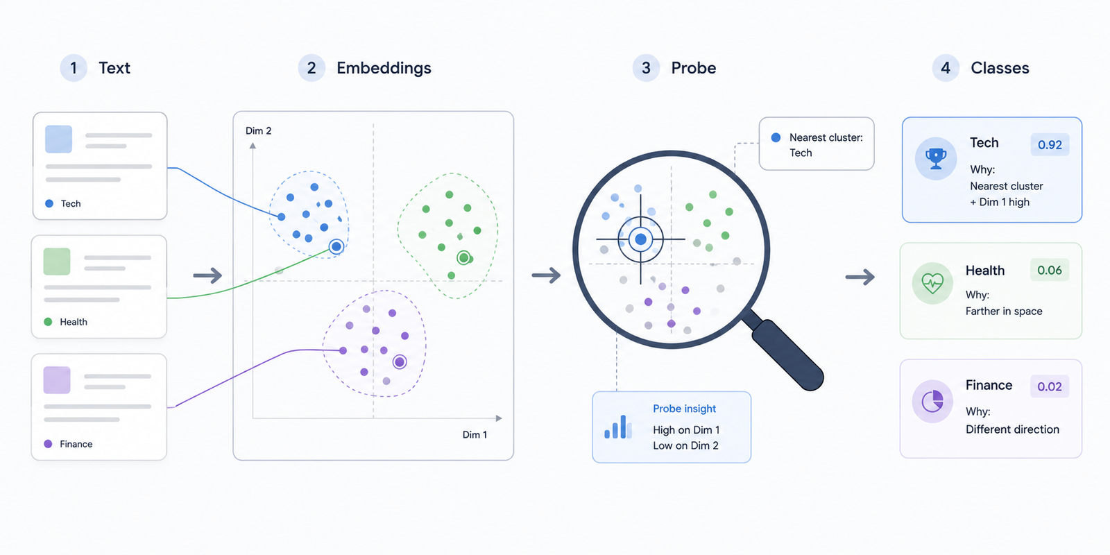
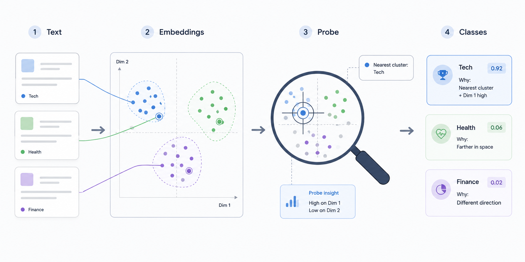
On this article, you’ll learn to use probing classifiers, UMAP visualization, and SHAP values to interpret and analyze the standard of textual content embeddings generated by massive language fashions.
Matters we are going to cowl embody:
- generate textual content embeddings from film critiques utilizing Scikit-LLM and a neighborhood Ollama mannequin, and practice a probing logistic regression classifier to guage their high quality.
- use UMAP dimensionality discount to visually examine the semantic construction captured by LLM-generated embeddings.
- apply SHAP values to determine which latent embedding dimensions have the best affect on a classifier’s predictions.
Introduction
Textual content classification duties have lengthy been solely the area of machine studying fashions and their direct “advanced kind”: deep neural networks. Nonetheless, we will’t deny that giant language fashions (LLMs) have revolutionized the best way textual content classifiers are actually constructed, being extra highly effective and correct however elevating a aspect concern: the dearth of interpretability as a result of LLMs being black-box fashions. Accordingly, when utilizing an LLM earlier than the core textual content classification job to transform uncooked textual content into embeddings — dense numerical vector representations of textual content — it’s doable to seize semantic data. But one difficult query arises: what precisely is the mannequin studying about textual content, and the way does this inner studying course of drive predictions?
This hands-on article reveals how you can use Scikit-LLM to generate embeddings, practice a probing classifier, and unveil the black field by leveraging UMAP visualization and SHAP (SHapley Additive exPlanations) values: two in style explainable AI methods for explaining mannequin inference and selections.
Preliminary Setup
The offered code right here is totally appropriate with Google Colab notebooks and requires putting in the most recent Scikit-LLM model. To maintain the entire course of cost-free, the code beneath reveals how you can configure all the pieces for native, free execution. Let’s begin by putting in the next dependencies and packages, together with the Ollama distributions for operating native LLMs at no cost:
|
# 1. Putting in Python libraries !pip set up –q scikit–llm umap–be taught shap
# 2. Repair Colab’s lacking system dependencies first (version-dependent, use with care in different environments) !apt–get replace –qq && apt–get set up –y –qq zstd
# 3. Putting in Ollama safely (because of zstd put in earlier) !curl –fsSL https://ollama.com/set up.sh | sh
# 4. Beginning the native server within the background and ready for it as well !nohup ollama serve > ollama.log 2>&1 & !sleep 5
# 5. Pulling the free embedding mannequin: all-minilm !ollama pull all–minilm |
Now let’s import all the pieces we are going to want:
|
import numpy as np import pandas as pd import matplotlib.pyplot as plt import umap import shap from skllm.config import SKLLMConfig from skllm.fashions.gpt.vectorization import GPTVectorizer from sklearn.model_selection import train_test_split from sklearn.linear_model import LogisticRegression from sklearn.metrics import classification_report from datasets import load_dataset |
Probing Embedding Areas
Step one to probe and analyze Scikit-LLM embeddings is, in fact, to get a recent assortment of them from a textual content dataset. We are going to first configure Scikit-LLM to level to a neighborhood Ollama server through "http://localhost:11434/v1/".
|
# 1. Pointing Scikit-LLM to the native Ollama server operating within the background SKLLMConfig.set_gpt_url(“http://localhost:11434/v1/”) SKLLMConfig.set_openai_key(“dummy_key”) # Required format, however ignored domestically |
After that, we use the general public IMDB dataset containing film critiques and cargo 1,000 of them: 500 labeled as optimistic and 500 labeled as destructive, giving us a superbly class-balanced pattern. We use stratified sampling to maintain 80% of the examples for coaching and the remaining 20% for testing:
|
1 2 3 4 5 6 7 8 9 10 11 12 13 14 15 16 17 |
# 2. Load one thousand film critiques from IMDB dataset print(“Downloading and getting ready IMDB dataset…”) dataset = load_dataset(“stanfordnlp/imdb”, cut up=“practice”) df = dataset.to_pandas()
# Extracting 500 optimistic and 500 destructive critiques to make sure an ideal steadiness df_pos = df[df[‘label’] == 1].pattern(500, random_state=42) df_neg = df[df[‘label’] == 0].pattern(500, random_state=42) df_balanced = pd.concat([df_pos, df_neg]).pattern(frac=1, random_state=42) # Shuffle
texts = df_balanced[‘text’].tolist() labels = df_balanced[‘label’].values
# Splitting through stratified sampling X_train, X_test, y_train, y_test = train_test_split( texts, labels, test_size=0.2, random_state=42, stratify=labels ) |
We are actually prepared for the heaviest a part of the method: producing embeddings for these 1,000 texts. We achieve this utilizing Ollama’s all-minilm mannequin through Scikit-LLM’s class designed for dealing with embedding fashions: GPTVectorizer. The syntax is deliberately just like customary scikit-learn information transformations, as we will see:
|
# 3. Producing Embeddings utilizing Scikit-LLM print(“Producing Embeddings…”) vectorizer = GPTVectorizer(mannequin=“all-minilm”) X_train_vec = vectorizer.fit_transform(X_train) X_test_vec = vectorizer.remodel(X_test) |
Be affected person; if you’re operating this on Colab, it might take about 5–10 minutes to finish, as we’re making 1,000 calls to a neighborhood LLM for embedding era.
A probing classifier (or a probing mannequin) is a diagnostic software used to examine the inner representations constructed by advanced fashions. How can we reliably decide that the embeddings generated earlier have sufficient high quality to separate the information into courses — optimistic vs. destructive critiques — correctly? A method is to make use of a smaller, less complicated classifier, comparable to logistic regression, and look at the accuracy metrics. If a classification report — described by precision, recall, and F1 scores per class — yields first rate outcomes even for this shallow classifier, that signifies the embeddings are wealthy sufficient for the classification job. Utilizing a less complicated classifier as our probing mannequin additionally helps isolate the contribution being attributed to the embeddings themselves.
|
# 4. Coaching the Probing Classifier print(“nTraining Classifier…”) clf = LogisticRegression(random_state=42, max_iter=1000) clf.match(X_train_vec, y_train) print(classification_report(y_test, clf.predict(X_test_vec))) |
Outcomes:
|
Coaching Classifier... precision recall f1–rating assist
0 0.77 0.76 0.76 100 1 0.76 0.77 0.77 100
accuracy 0.77 200 macro avg 0.77 0.77 0.76 200 weighted avg 0.77 0.77 0.76 200 |
Contemplating that the dataset dimension just isn’t terribly massive relative to the embedding dimensionality, these outcomes are fairly respectable for a easy, linear classifier like logistic regression, which is often utilized to smaller, purely tabular datasets.
Let’s have a look at one other introspection software: UMAP (Uniform Manifold Approximation and Projection). UMAP is a projection-based dimensionality discount method generally used for visualization. We challenge the embeddings right down to 2 dimensions utilizing cosine similarity as the space metric, which is customary when working with textual content embeddings. The ensuing scatterplot helps us decide whether or not there’s any pure grouping between embeddings related to optimistic and destructive critiques:
|
1 2 3 4 5 6 7 8 9 10 11 12 13 14 15 16 17 18 19 20 21 22 23 |
# 5. Visualize with UMAP print(“Working UMAP Projection…”) reducer = umap.UMAP( n_components=2, metric=‘cosine’, # Native metric for transformer embeddings n_neighbors=30, # Captures broader international construction min_dist=0.1, # Prevents extreme level overlap random_state=42 ) X_umap = reducer.fit_transform(X_train_vec)
plt.determine(figsize=(9, 6)) scatter = plt.scatter( X_umap[:, 0], X_umap[:, 1], c=y_train, cmap=‘coolwarm’, s=25, # Smaller marker dimension alpha=0.6, # Transparency reveals true density edgecolors=‘none’ # Eliminates border muddle ) plt.title(“UMAP Projection of Scikit-LLM Embeddings”) plt.present() |
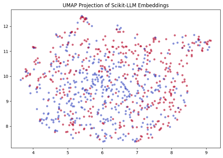
The outcomes will not be extraordinary at first look — there isn’t any near-perfect class-wise separation between critiques — however contemplating these are LLM-generated embeddings closely projected into simply two dimensions, a refined sense of grouping remains to be seen: the southern half of the plot reveals a dominance of destructive critiques (blue dots), whereas the higher half has a majority of optimistic critiques (fuchsia).
Final, we will resort to one of the crucial in style frameworks for analyzing machine studying mannequin habits: SHAP (SHapley Additive exPlanations). SHAP may also help us perceive which of the latent dimensions (options) in our embeddings had essentially the most affect on the probing classifier’s predictions.
The code beneath constructs a SHAP abstract plot that visualizes which embedding dimensions exert essentially the most influence on mannequin classifications. By default, the plot shows the highest 20 options with the most important total influence, utilizing coloration to point whether or not every characteristic contributes towards optimistic or destructive classifications relying on whether or not its values are larger or decrease.
|
1 2 3 4 5 6 7 8 9 10 11 12 13 14 15 16 17 18 |
# 6. Extracting Characteristic Significance with SHAP print(“Calculating SHAP values…”) explainer = shap.LinearExplainer(clf, X_train_vec) shap_values = explainer.shap_values(X_test_vec)
# Standardizing SHAP output format throughout totally different scikit-learn variations if isinstance(shap_values, checklist): shap_values = shap_values[1]
plt.determine(figsize=(8, 5)) shap.summary_plot( shap_values, X_test_vec, feature_names=[f“Dim {i}” for i in range(X_train_vec.shape[1])], present=False ) plt.title(“SHAP Abstract: Most Impactful Latent Dimensions”) plt.present() |
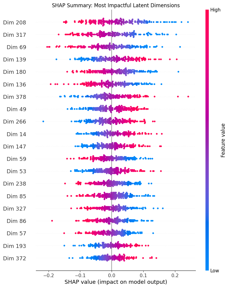
We will conclude that dimension 208 is the first sign for destructive critiques, carefully adopted by dimension 317. In the meantime, dimension 139 is the principle driver for optimistic critiques, as larger values (pink) for this characteristic push the mannequin’s uncooked prediction towards larger values (the right-hand aspect of the plot, leaning towards the optimistic class).
Conclusion
This text illustrated how you can use a probing classification mannequin, together with visualization instruments like UMAP and SHAP, to raised perceive and interpret the character and high quality of textual content embeddings produced by LLMs for downstream machine studying duties like textual content classification. We relied on Scikit-LLM, a library that mirrors scikit-learn’s API to seamlessly combine LLMs into a wide range of duties, together with embedding era from uncooked textual content comparable to film critiques.