How Unsuitable Is Your Advertising Combine Mannequin (MMM)?

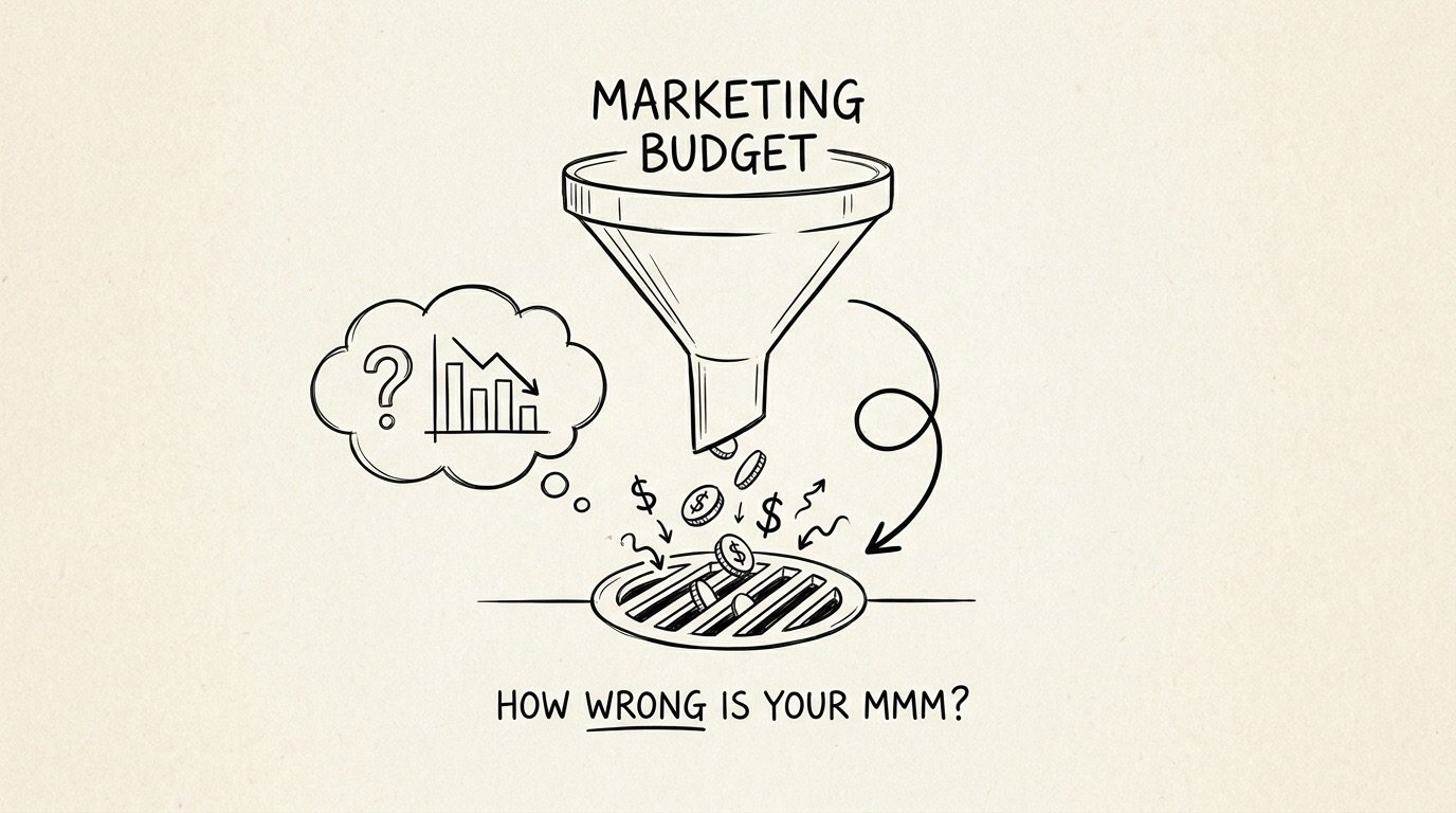
Measuring the return on advertising spend is among the hardest jobs in development, however Advertising Combine Modelling has had a resurgence as the reply to it in recent times. Open-source releases have pushed most of that: Robyn from Meta, Meridian from Google, PyMC-Advertising from PyMC Labs. Working an MMM has by no means been simpler. Trusting one is a unique query.

Google set out why again in 2017, in Challenges and Alternatives in Media Combine Modeling, a paper that’s nonetheless the clearest assertion of what goes flawed. Three of the issues it names do many of the harm. Each comes from a unique type of variation that’s lacking out of your spend.

• Multi-collinearity. Advertising channels get set in the identical planning cycle, so that they rise and fall collectively. No mannequin can separate channels that by no means moved aside, so the estimates come again with excessive variance. What’s lacking is every channel transferring by itself.

• Choice bias. Spend follows demand, with organisations spending extra on advertising in peak durations. However as demand itself is not immediately observable, the mannequin has to fall again on proxies for it. The channel coefficients take in what these proxies miss: textbook omitted variable bias. What’s lacking is spend that strikes for causes apart from demand.

• Non-identifiable adstock and saturation. Each MMM additionally has to establish adstock and saturation results. A 2024 examine titled Your MMM is Damaged discovered these form parameters are sometimes not individually identifiable from odd spend knowledge both. What’s lacking is spend at clearly completely different ranges, held for lengthy sufficient to outlast the carryover.

Google’s 2017 paper’s personal reply was higher knowledge. Almost a decade on, the trade’s principal response has been incrementality testing, now more and more used to calibrate MMMs. That’s actual progress, however it reads one channel at a time and may take months to get a dependable impression. And a 2026 Recast examine discovered most open-source geo-testing instruments report a false carry 14-30% of the time.

Step again and all three issues have the identical repair: spend that varies within the methods the mannequin wants. This simulation examine asks whether or not a finances phasing algorithm can construct all three sorts of variation right into a plan.

1. Information producing course of

No person is aware of how a lot income every channel really drove final yr. We additionally do not understand how a lot income every channel will drive subsequent yr given your deliberate finances. Subsequently, to check whether or not a finances phasing algorithm helps, we’d like an information producing course of the place we all know the bottom fact. We are able to obtain this by simulating income from a recognized response to advertising, giving us one thing to validate our mannequin estimates in opposition to. That is pretty widespread observe relating to assessing how good your MMM is, however right here we’re utilizing it to evaluate the impression of a finances phasing algorithm.

Step 1: Simulate advertising spend and demand

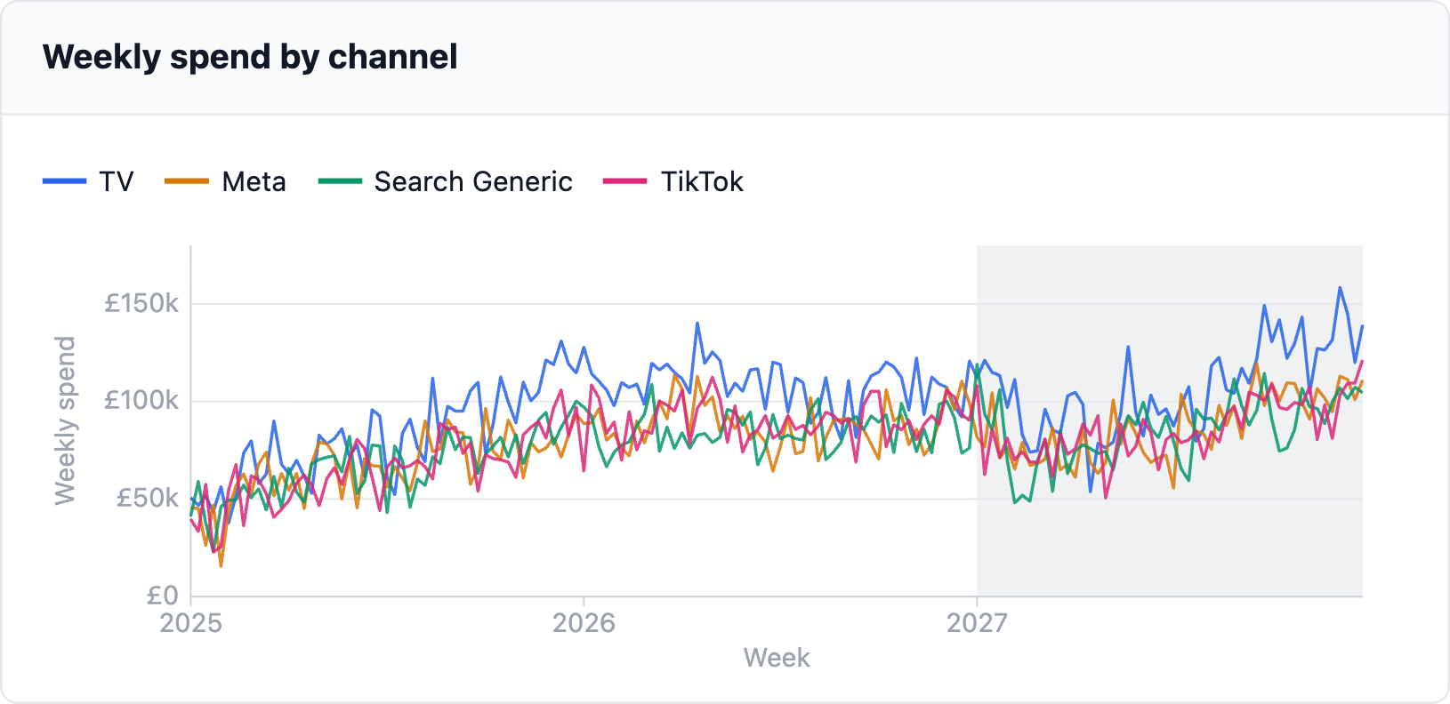
We generate three years of weekly spend for TV, Meta, Search Generic and TikTok. In actuality you almost certainly have greater than 4 channels, however we select 4 channels for example the issue and discover the answer, after which reveal whether or not it could scale to 10-15 channels later within the article. We select three years of weekly spend knowledge as it is a widespread alternative in MMM, because it balances the trade-off between having sufficient knowledge and conserving it latest. The channels all comply with the identical underlying sign, which supplies them a correlation coefficient of 0.7. The correlation coefficient is excessive, however it is a practical state of affairs pushed by finances planning following demand forecasts. Later within the article we additionally discover the impression of various correlation coefficients. That shared sign traits upward, so spend drifts up over the three years. Take note we simulate spend for the aim of this text. In observe you provide your final two years of precise spend and subsequent yr’s plan, which collectively make up the three years an MMM is usually skilled on.

Gross sales rely on greater than advertising. Underlying demand, how a lot folks would purchase in a given week no matter promoting, drives gross sales too. As a result of budgets are deliberate round it, it additionally strikes with spend, and that’s the place choice bias comes from.

No person observes demand immediately, so we assemble it: a sequence that strikes with the spend at a correlation of 0.65. That determine is an assumption, since spend knowledge cannot reveal the true worth. With your personal knowledge, the bundle builds demand out of your actual spend in the identical approach.

Spend explains slightly over half of demand at these settings. The remainder follows one in all 5 patterns:

• Development: drifts steadily up or down. Our default.

• White noise: jumps randomly every week, with no sample.

• Gradual drift (AR(1)): wanders, with every week staying near the final.

• Seasonal: repeats the identical sample yearly.

• Seasonal with drift (seasonal AR(1)): a yearly sample plus gradual wandering.

With your personal knowledge, decide the sample closest to how your gross sales behave other than advertising: regular development, a robust yearly cycle, or neither.

Step 2: Select the response

Earlier than we will generate gross sales/income, we have to arrange the response operate for advertising channels. Every channel will get a marginal return, a saturation curve (how shortly additional spend stops paying again) and an adstock decay (how lengthy an advert retains working after the week it runs). For the aim of this text we use believable values, however in observe you must use the outcomes out of your MMM. That may appear round, however the purpose is practical gross sales knowledge the place the true response is understood. That lets us measure how a lot harm correlated spend does, and the way a lot finances phasing repairs.

The state of affairs used all through this text

Marginal return is the income the following £1 brings in on the channel’s deliberate weekly spend: £0.50 for TV and £1.50 for Search Generic. To maintain issues easy we use a power-curve saturation and geometric adstock, however this may be tailored to match the response you might be utilizing in your MMM. Saturation is the exponent on spend: 1.0 is a straight line, and the decrease the worth, the quicker additional spend stops paying again. Adstock is the share of an advert’s impact that carries into the following week, so TV retains half and Search Generic retains a tenth. The response operate additionally requires an assumption for baseline, what gross sales can be with no advertising. We use a believable worth of 70%, however once more you must use the worth out of your MMM outcomes.

Each variance and bias determine on this article is conditional on these inputs. They present what a mannequin would get flawed if the world labored this manner. They aren’t a measurement of your personal MMM.

Step 3: Generate gross sales/income

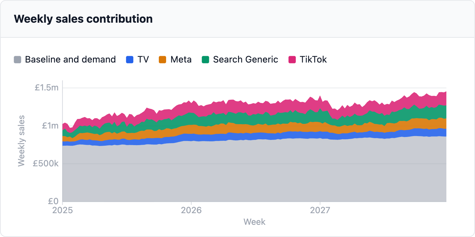
We now have all of the elements to generate gross sales:

• Channel contributions. How a lot every channel contributes to gross sales utilizing marginal return, adstock and saturation.

• Baseline. What gross sales can be with no advertising.

• Demand. A hidden weekly sequence for the whole lot exterior your advertising that strikes gross sales, reminiscent of seasonality or the financial system. It’s what makes your baseline rise and fall. We measurement it so the baseline varies by 5% round its common. You possibly can provide this from your personal MMM: take its baseline sequence and divide its customary deviation by its imply.

• Demand proxy. We won’t observe demand immediately, however we will use a proxy reminiscent of a class search index. How intently a proxy tracks demand cannot be measured both, so we assume a correlation of 0.8.

• Noise. Random week-to-week variation that nothing within the mannequin explains, with a normal deviation of two% of common weekly gross sales. That is pure noise: demand, together with the half a proxy misses, is modelled individually above. Every simulation redraws it, which exhibits how far the estimates transfer throughout believable variations of the identical historical past.

Now that now we have an acceptable knowledge producing course of, we will begin by assessing the issue. After we use our generated knowledge to construct an MMM, what’s the variance and bias, and the way identifiable are adstock and saturation?

2. Three separate methods your mannequin can mislead you

Now let’s transfer on to assessing the issue. There are three areas we’re going to deal with:

• Variance. When you refit your MMM on a barely completely different model of the identical historical past, how far would its reply transfer?

• Bias. Throughout all these refits, does the common reply land on the reality, or is it persistently off to 1 aspect?

• Identifiability. Can the mannequin get well every channel’s adstock and saturation?

Drawback 1: Variance

We simulate 50 gross sales sequence from the information producing course of. Each retains the spend, the response and demand mounted and solely redraws the noise, so every is a model of the identical three years that would equally have occurred. We match an MMM to every sequence, giving it the true demand and the true curve shapes, so the one factor that may make the estimates differ is noise assembly correlated spend. That could be a finest case: an actual MMM has to estimate these too, so its estimates would transfer a minimum of this a lot. We then evaluate every channel’s estimated incremental income on subsequent yr’s plan with the bottom fact.

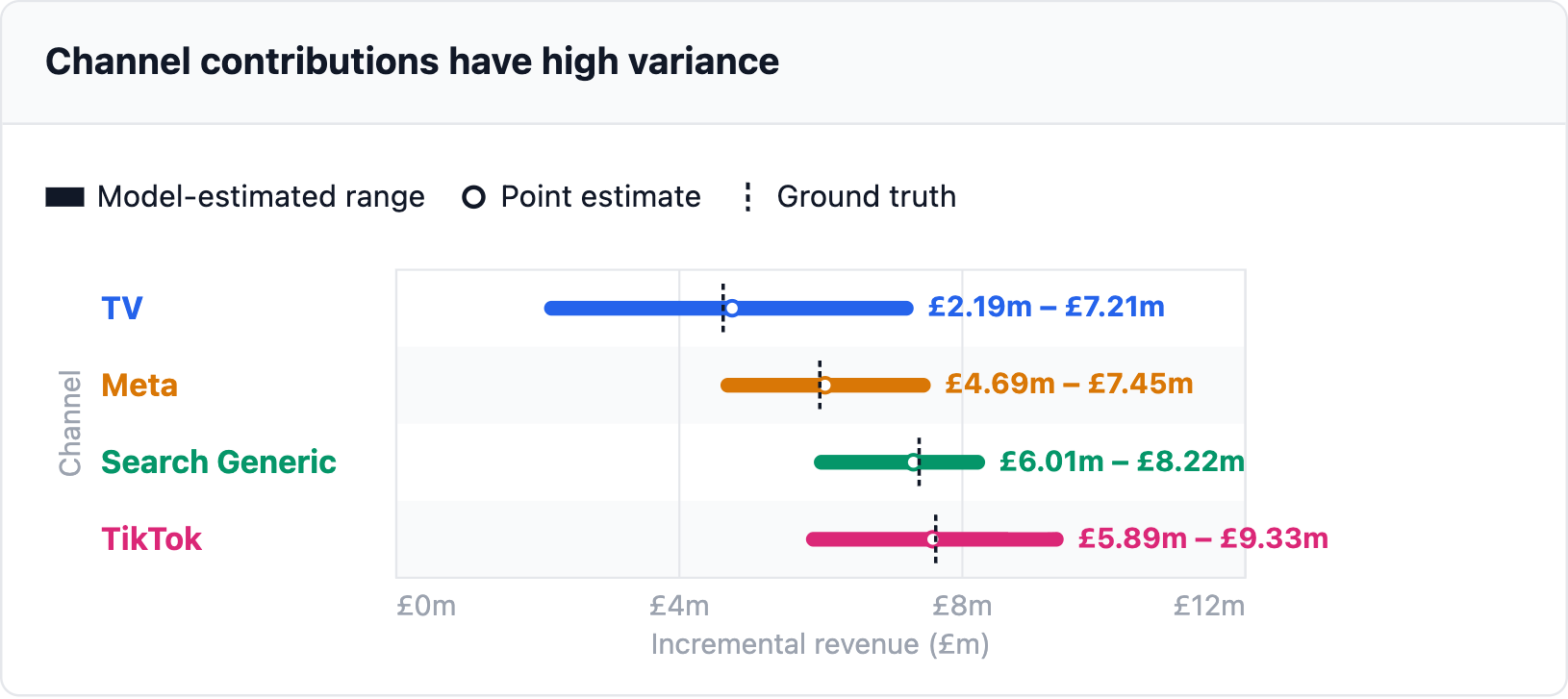
Look intently at how huge these ranges are. Any one of many 4 channels may have the best incremental income. This is not bias: with correlated channels the regression nonetheless lands on the reality on common, so long as the mannequin is specified appropriately. The issue is that three years of weekly knowledge include little or no impartial motion per channel, so any single match, together with yours, may land wherever in that vary.

Drawback 2: Bias

We match the identical approach as for variance, with one change: the mannequin will get the demand proxy as a substitute of the true demand, simply as an actual MMM would. How massive the bias is depends upon the actual demand sequence and proxy we occur to attract, so a single draw may flatter or exaggerate it. We subsequently draw 100 variations of demand and its proxy, run the 50 simulations on every, and evaluate the common estimate with the bottom fact.

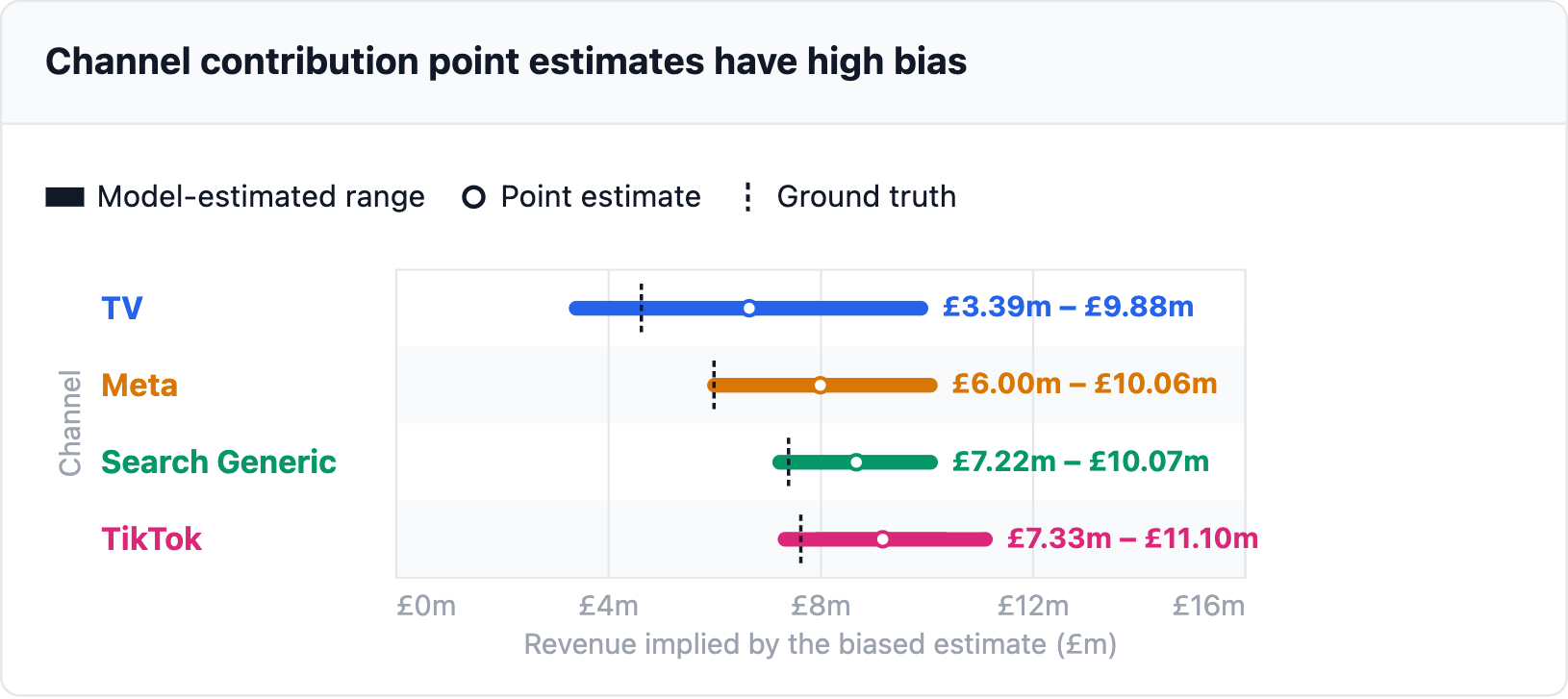
Take note of how the purpose estimates sit above the bottom fact for each channel: TV by 44%, Meta by 33%, TikTok by 20% and Search Generic by 17%. That is pushed by spend following demand. When demand lifts gross sales, spend is up too, and regardless of the proxy misses will get credited to the channels. That is omitted variable bias, and in contrast to variance it does not common out with extra knowledge. Refitting the identical mis-specified mannequin on extra weeks simply will get you a tighter estimate of the flawed quantity.

Drawback 3: Identifiability

We simulate 50 gross sales sequence with contemporary noise and provides the mannequin the true demand. We then take one channel at a time. The opposite channels hold their true saturation and adstock, and for the one being examined we attempt each mixture of saturation exponent (0.20 to 1.00) and adstock decay (0.00 to 0.90) and hold the one that matches finest. The unfold of these most closely fits throughout the 50 sequence is the recovered vary. It is a finest case too: an actual MMM has to estimate each channel’s form without delay.

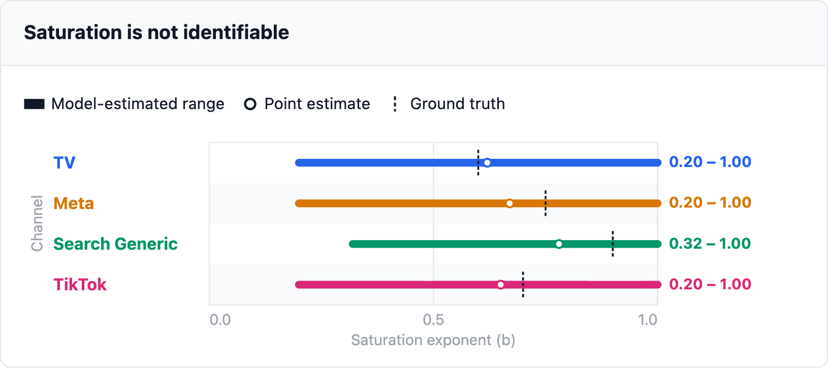
Saturation fares worst. For 3 of the 4 channels the vary covers the entire 0.20 to 1.00 search. The mannequin cannot inform TV’s bending curve (true 0.60) from a straight line, as a result of seeing curvature wants a channel noticed at clearly completely different spend ranges whereas the others maintain nonetheless. Right here each channel rises and falls collectively, so a straight line and a curve match the information about equally effectively.

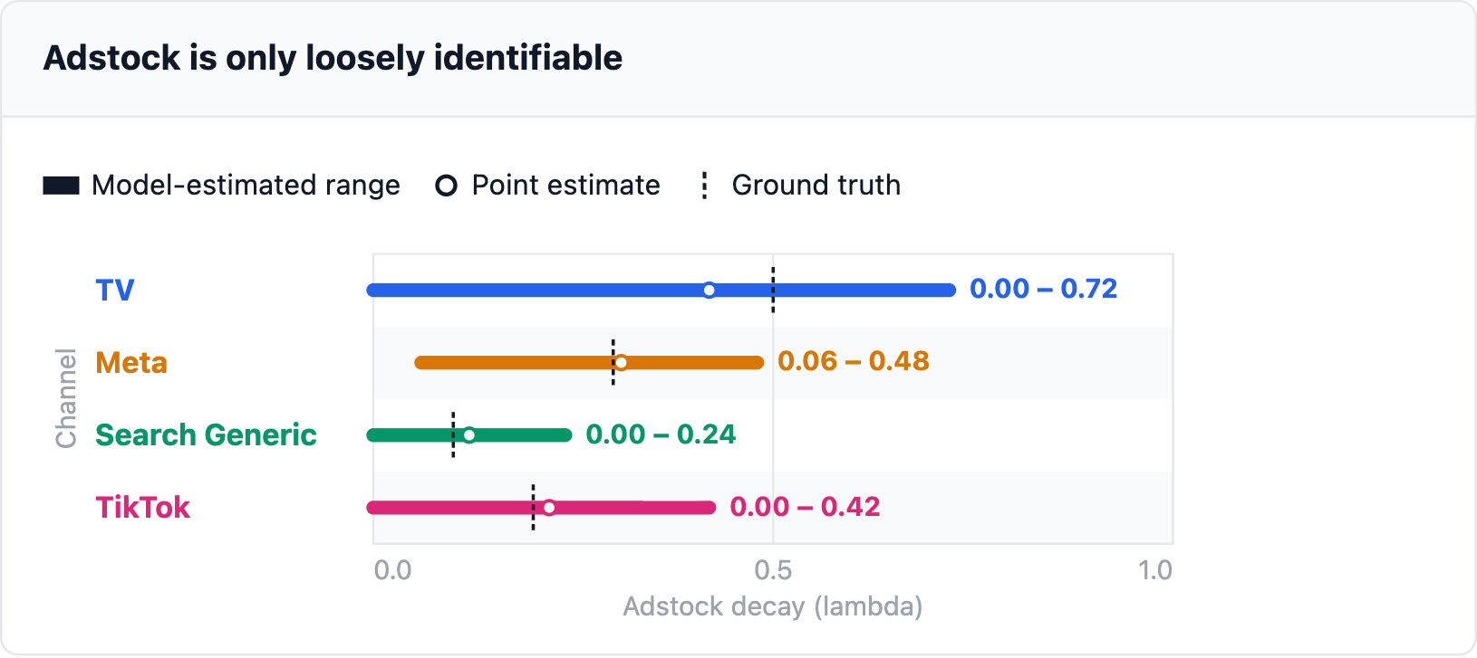
Adstock is healthier however nonetheless huge: each channel’s vary reaches zero or near it, so the mannequin cannot rule out that advertisements cease working the week they run. TV’s true decay is 0.50, but its vary runs from 0.00 to 0.72.

Most groups reply to any one in all these three issues by tweaking the mannequin: completely different priors, completely different transformations, a unique baseline or curvature specification. That hardly ever helps, as a result of the mannequin is not the issue. Channels that all the time moved collectively cannot be advised aside by any estimation technique, nevertheless subtle. Within the subsequent part we are going to dig slightly deeper into the trigger.

3. Your channels by no means transfer on their very own

This is why the mannequin is so uncertain on all three counts. TV, Meta, Search Generic and TikTok budgets get set in the identical planning cycle, so when one goes up, they often all go up. In our knowledge producing course of each pair of channels has a correlation between 0.60 and 0.68.

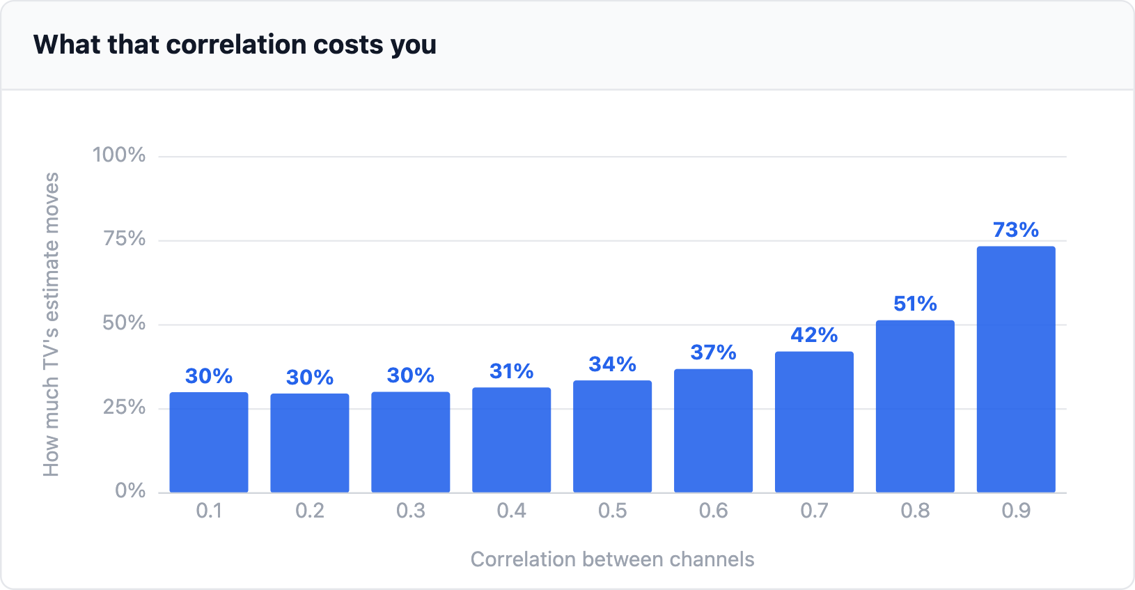
To see what that correlation prices, we rerun the variance measure from part 2 at each correlation from 0.1 to 0.9. All the things else is held mounted: the identical finances and demand, the identical response and the identical week-to-week unfold in spend. We monitor TV’s coefficient of variation: how a lot its estimated incremental income strikes throughout refits, as a share of the estimate.

Even when the channels moved utterly independently TV’s estimate would nonetheless transfer by about 30% of itself. That flooring comes from gross sales noise and the quantity of knowledge slightly than correlation. Correlation provides to it: 42% at our 0.7 and 73% at 0.9.

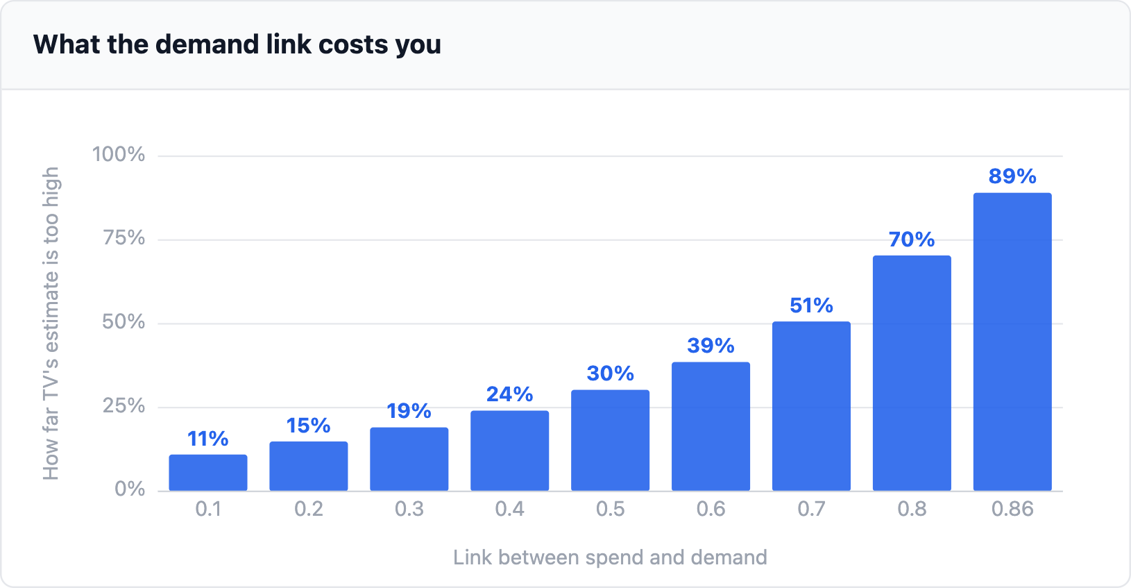
Bias works in another way. It depends upon how intently spend follows demand slightly than how intently channels comply with one another. So right here we maintain the channels at 0.7 and sweep the hyperlink between spend and demand as a substitute (0.65 in our knowledge producing course of).

Even with a weak hyperlink of 0.1 TV’s estimate is 11% too excessive. At our 0.65 it’s 44% too excessive and at 0.86 it’s 89% too excessive. 0.86 is the strongest hyperlink doable when the channels sit at 0.7.

Adstock and saturation are a unique type of drawback. Each want one thing from the spend itself. Adstock wants a change that’s held for longer than the carryover lasts. Saturation wants spend at a number of clearly completely different ranges. So there are three causes slightly than one, and a repair has to provide a unique type of variation for every.

It is not that the mannequin is badly constructed. It is that the information it is studying from was by no means designed to reply any of those three questions.

4. Identical finances, a wiser phasing algorithm

You do not want a much bigger mannequin, a much bigger finances, or an AI agent bolted onto your MMM. You want spend that carries extra data, and a phasing algorithm can provide it. Which means every channel transferring by itself, for causes that don’t have anything to do with demand. It additionally means spend at a number of ranges, every held for lengthy sufficient to register.

The concept is not new. MMM distributors already say it: Recast inform purchasers to deliberately fluctuate spend so the mannequin turns into identifiable, and go-dark checks have been round for years. What has been lacking is the how a lot. Which channel to maneuver, by how far, and what you get again for it. This part goes into completely different phasing methods, why we selected them and which works finest.

What phasing has to do

Part 3 confirmed that every drawback wants one thing completely different from the information. A phasing technique has to provide it.

• Variance. Every channel has to maneuver in weeks when the others do not. Random strikes, drawn individually for every channel, do that.

• Bias. The strikes will need to have nothing to do with demand. A schedule drawn at random earlier than the yr begins cannot comply with it.

• Adstock. A change must be held for longer than the carryover lasts. Adstock smooths away a one-week blip, however a darkish run or a month-long step survives it.

• Saturation. The channel wants spend effectively above its plan, held lengthy sufficient to outlast adstock. Going darkish does not assist right here: zero spend provides zero response regardless of the curve’s form.

The methods

We take a look at six methods. The primary three are constructing blocks, every aimed toward one of many jobs above. The fourth runs all three collectively. The final two are lighter alternate options.

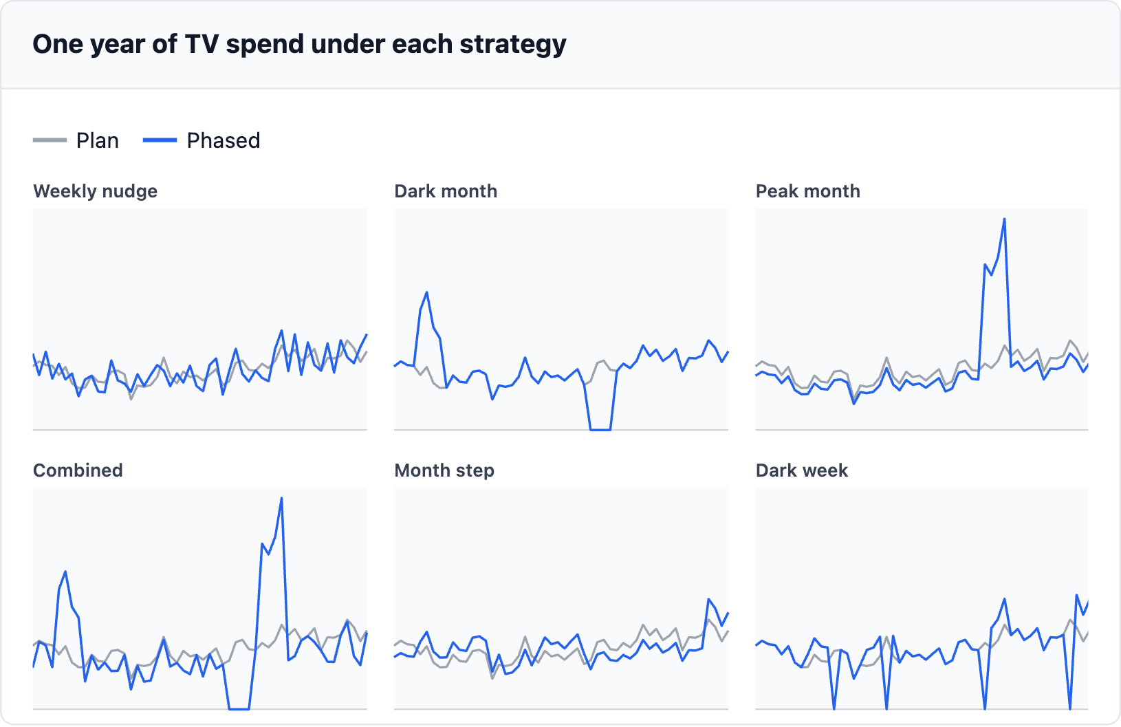
• Weekly nudge. Each week strikes up or down by 20%. Ups and downs are balanced inside the month, and the month is then rescaled to its deliberate complete, which may carry the most important week to 1.25 instances plan. It’s there for variance.

• Darkish month. Every year every channel goes darkish for 4 weeks in a row. That finances strikes into one different month. Channels take turns, so with as much as 12 channels no two go darkish in the identical month. It’s there for bias and adstock.

• Peak month. One month a yr runs at 2.5 instances plan. A small equal reduce to the channel’s different months pays for it. Channels take turns, so with as much as 12 channels no two peak in the identical month. It’s there for saturation.

• Mixed. All three collectively: the darkish month, the height month, and the weekly nudge in each different month.

• Month step. Every complete month strikes up or down by 20%. Each channel will get six up months and 6 down months. No two channels comply with the identical sample.

• Darkish week. One week 1 / 4 goes darkish, in a month picked at random. The remainder of that month absorbs its finances.

Each technique is drawn individually for every channel and retains every channel’s annual finances. Weekly nudge and darkish week additionally hold each month’s complete. The opposite 4 transfer cash between months.

We additionally tried two different weekly nudges: random sizes as much as 20% and strict alternation between up and down. Neither improved on the fixed-size nudge, so they’re overlooked.

Which works finest

We run each technique via the measures from part 2 and evaluate it with the unphased plan. Every technique is averaged over 15 random attracts of its schedule, and bias over 100 attracts of demand.

The six methods on this state of affairs

How you can learn the columns. Decrease is healthier in each one:

• Variance: the coefficient of variation, averaged over the 4 channels.

• Bias: the imply absolute % hole from the reality, averaged over the 4 channels.

• Saturation and adstock: the common width of every channel’s vary from part 2.

• Price: the share of the income every channel drives within the plan yr that’s given up, averaged over the 4 channels.

• Peak: the most important single week as a a number of of its plan.

Every determine is a median over many simulated runs, so it might transfer slightly if we ran them once more. Deal with small gaps between methods as ties.

Mixed is finest on all 4 diagnostics. Variance falls from 0.23 to 0.07 and bias from 28.8% to fifteen.3%. The saturation vary greater than halves from 0.77 to 0.31 and the adstock vary falls from 0.45 to 0.18.

It additionally prices essentially the most. Darkish month is the closest various: it will get 92% of Mixed’s variance achieve and 71% of its bias achieve for about half the associated fee (1.82% in opposition to 3.42%). What it could’t do is pin down saturation as effectively, the place its vary is 0.40 in opposition to Mixed’s 0.31. Weekly nudge is the weakest: Month step beats it on variance and bias and is stage on the remainder, on the identical value.

Accuracy doesn’t come without cost. We predict Mixed’s additional accuracy is value its value, so it’s the technique we feature ahead. If that value is just too excessive for you, Darkish month is the place to start out.

What it prices

• Income given up. Returns diminish as spend rises, so finances moved from a quiet week right into a busy one earns lower than it did. The associated fee follows how far spend is pushed up the curve, the place every additional pound earns least. That can also be what pins saturation down.

• Platform studying phases. Advert platforms can re-enter a studying section after a big finances change and ship worse whereas they do. We do not mannequin this. It’s why the weekly nudges are capped at 20%. Darkish months and peak months are a lot larger strikes, which is why the height column issues.

Remember the fact that in our knowledge producing course of demand provides to gross sales and does not change how effectively media works. In case your media works more durable when demand is excessive, transferring spend out of busy weeks prices greater than we present.

5. What the phasing algorithm buys you, and what it prices

From right here on we deal with Mixed, the very best of the six methods on this state of affairs.

The phased plan

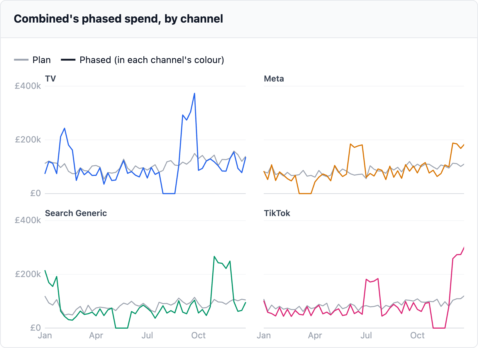
Every channel will get 4 darkish weeks and two months effectively above plan: the one which takes the darkish weeks’ finances and the height month. No two channels go darkish in the identical month. In each different month every week strikes up or down by 20%. Every channel’s annual finances is unchanged.

Correlation

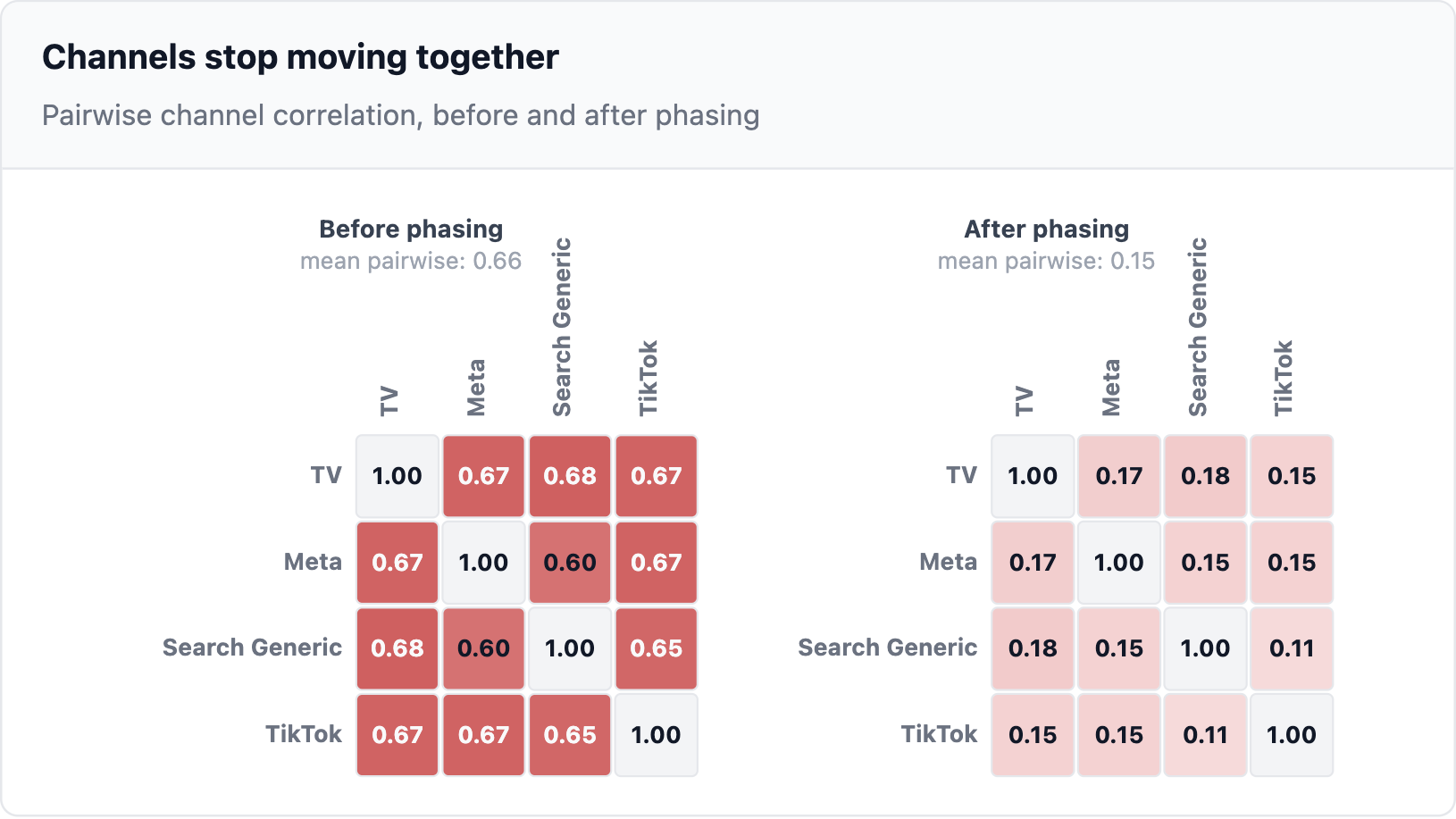
Earlier than phasing each pair of channels strikes collectively at between 0.60 and 0.68. After, each pair falls to between 0.11 (Search Generic/TikTok) and 0.18 (TV/Search Generic). Imply pairwise correlation falls from 0.66 to 0.15. Identical channels and the identical annual finances. Solely the timing modified.

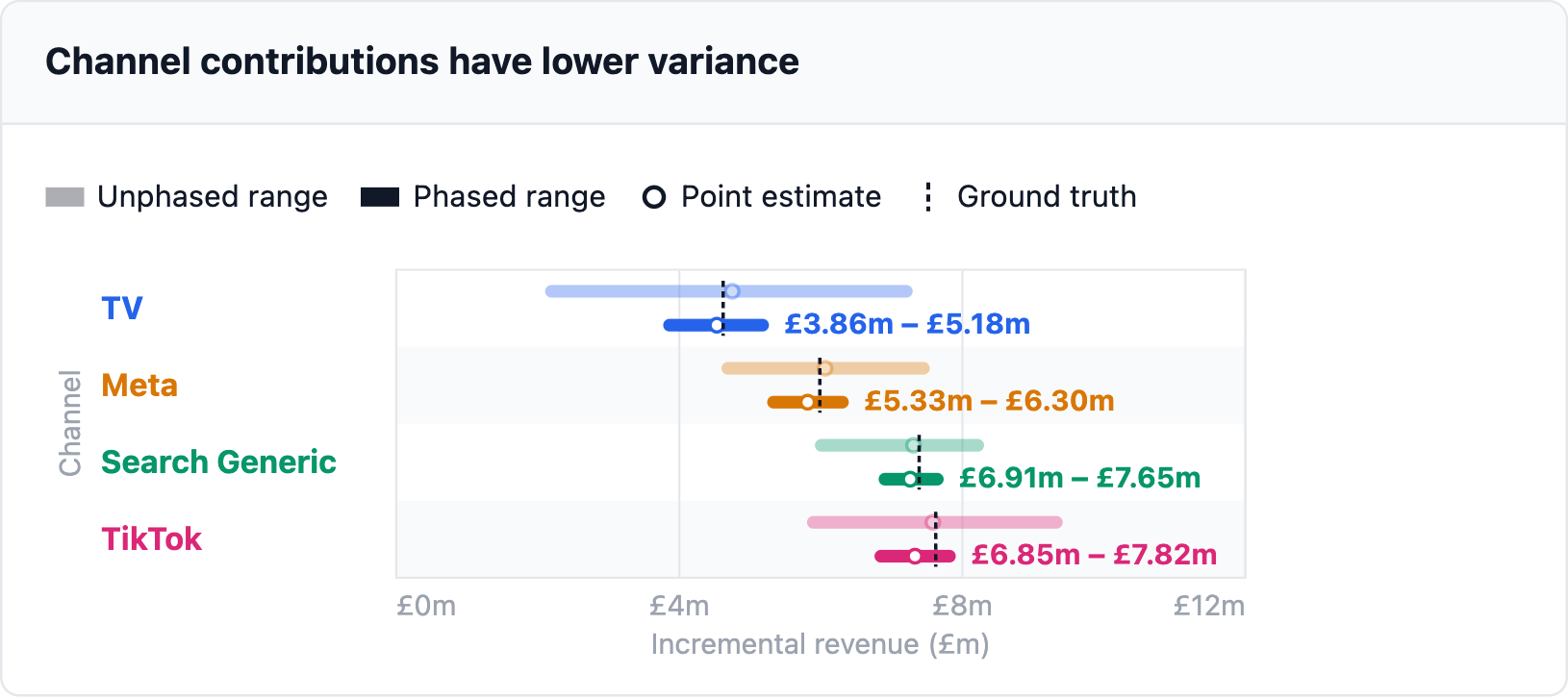
Influence 1: Variance

The vary narrows for each channel: by 65% for Meta as much as 74% for TV. The purpose estimate barely strikes as a result of variance is concerning the unfold, not the centre.

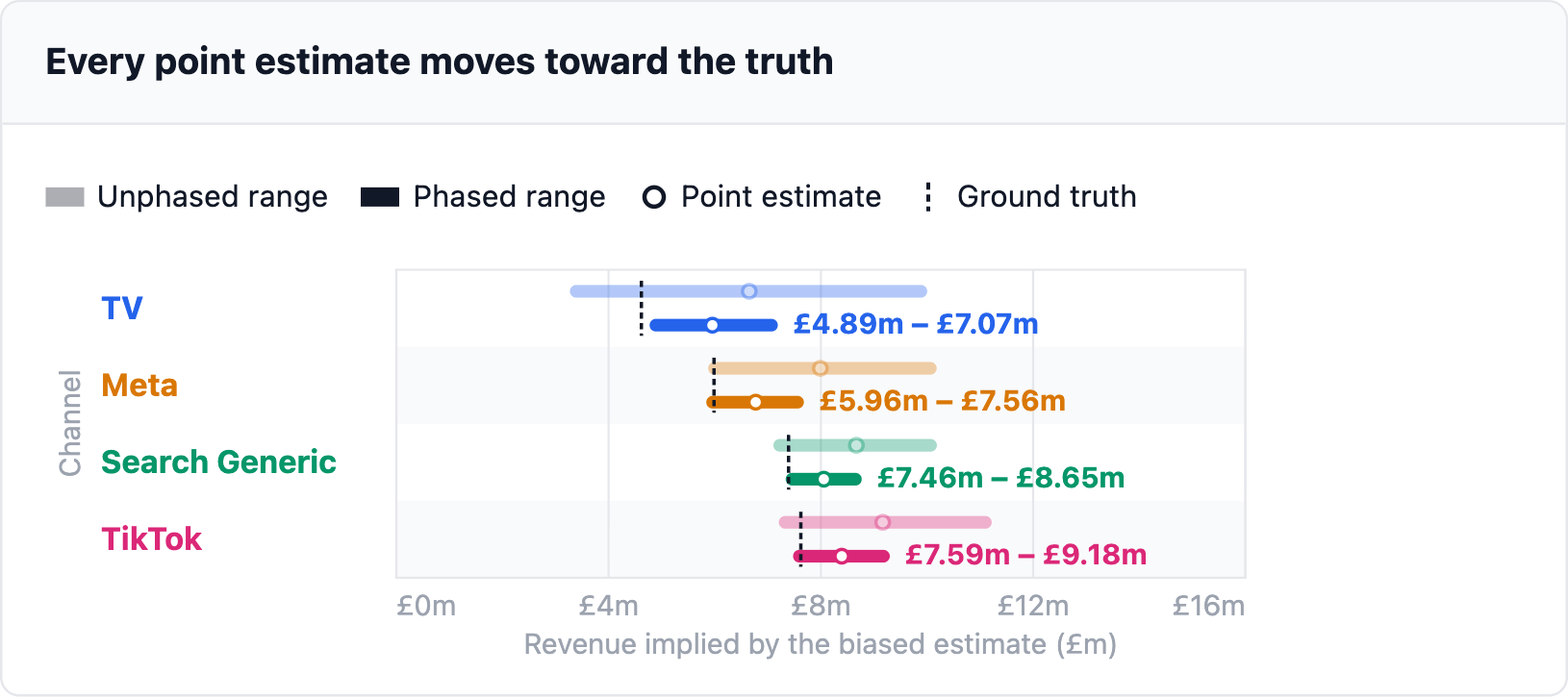
Influence 2: Bias

All 4 level estimates transfer towards the bottom fact. TV’s bias falls from 44.0% to 29.0%, Meta’s from 33.5% to 13.1%, TikTok’s from 20.2% to 10.1% and Search Generic’s from 17.3% to 9.0%.

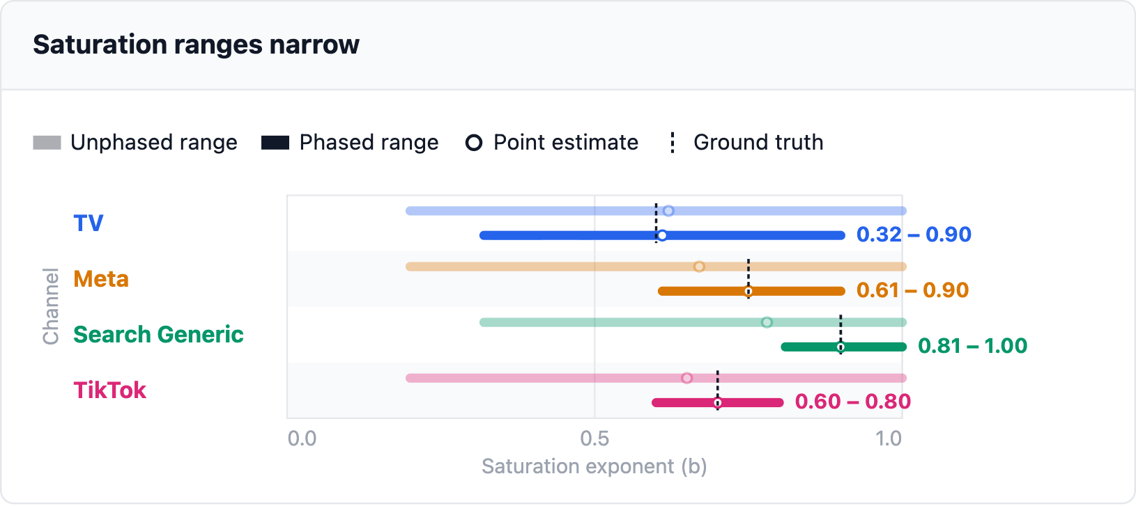
Influence 3: Identifiability

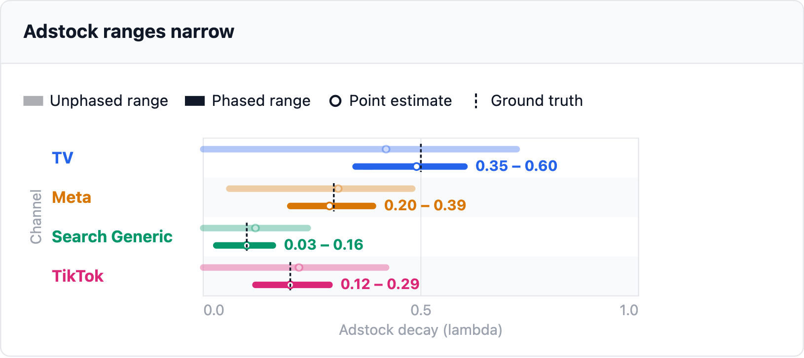
On saturation TV, Meta and TikTok not cowl the entire 0.20 to 1.00 search. TV narrows the least: its vary nonetheless runs from 0.32 to 0.90.

On adstock each vary tightens, and TV and TikTok not attain all the way down to zero. Search Generic was already tight and narrows slightly, from 0.00–0.24 to 0.03–0.16.

How the profit builds

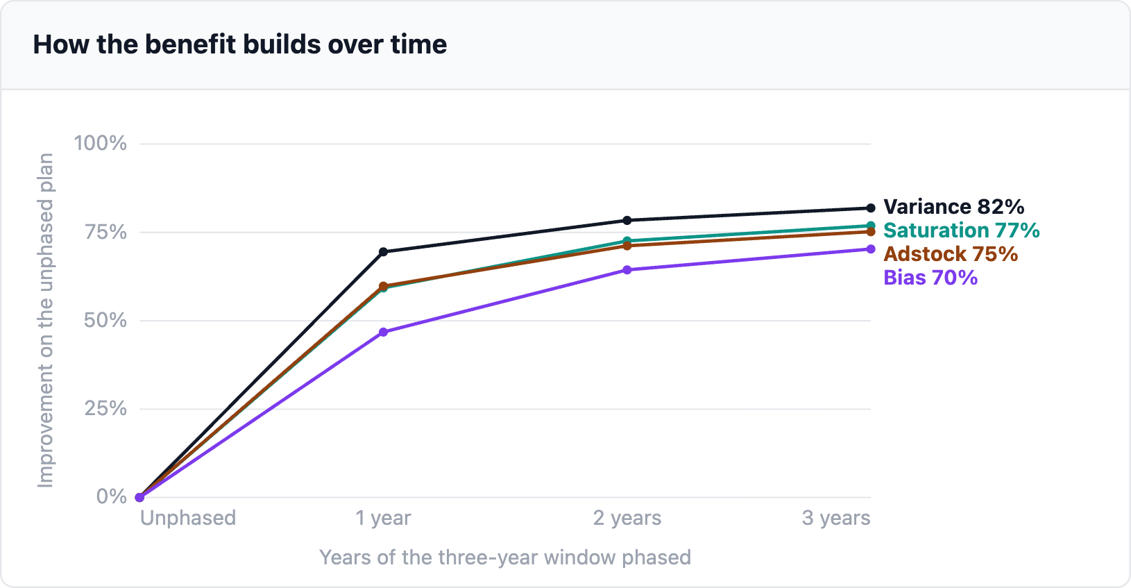
All the things above is after one yr of phasing. The mannequin is fitted on three years and solely the final of them is phased. If the phasing retains working the good points hold coming as extra of the three-year window is phased.

A lot of the achieve lands within the first yr. 12 months one delivers 85% of the three-year enchancment in variance, 77% for saturation and 80% for adstock. Bias improves the slowest: 47% higher after one yr and 70% after three. The traces flatten by yr three.

What it prices

Mixed provides up 3.42% of the income the 4 channels drive within the plan yr, the many of the six methods. That’s about £0.9m of £25.6m, or 1.5% of complete gross sales. The annual plan stays at £19.0m and no additional spend is required. Solely the timing modifications.

The associated fee depends upon the saturation curves, which part 2 confirmed are exhausting to pin down. Preserving the identical schedule and transferring each channel’s exponent throughout that vary, the associated fee runs from 0.3% when the curves are straight traces to five.3% at an exponent of 0.4.

6. Does it scale to all of my channels?

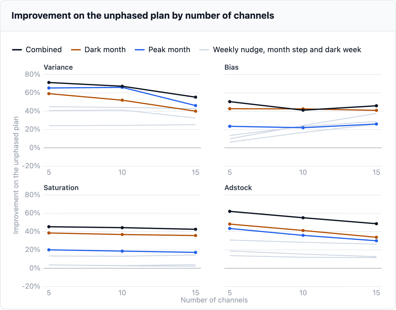
All the things thus far makes use of 4 channels. Most MMMs have greater than that, so on this part we take a look at whether or not the phasing algorithm nonetheless works at 5, 10 and 15 channels.

We hold the information producing course of from part 1 and solely change the variety of channels. Every added channel copies one of many 4 from part 1, and each pair nonetheless has a correlation of 0.7. The noise is held at its four-channel measurement. As a result of outcomes at 10 and 15 channels fluctuate from one simulated dataset to the following, each level is averaged over 4 of them.

The variance and adstock good points shrink as channels are added however maintain up. At 15 channels Mixed nonetheless cuts variance by greater than half and bias by almost half, and its saturation achieve barely strikes. Each technique stays forward of the unphased plan on each measure. The probably purpose for the shrinkage is that the identical three years of knowledge are unfold throughout extra channels.

7. One pipeline, three steps

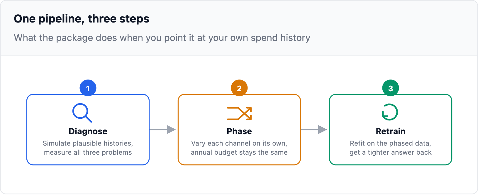
All of this runs via how_wrong_is_your_mmm, a free, open-source Python bundle. Level it at your personal spend historical past and it runs the identical three steps in your numbers, not a hypothetical instance.

Step 1: Diagnose

You provide your weekly spend historical past and plan by channel. You additionally provide values out of your MMM: every channel’s marginal return, saturation and adstock, plus the baseline, the noise and the way intently spend follows demand. The bundle simulates many believable variations of that historical past and refits an MMM on each. It measures variance, bias and the way identifiable adstock and saturation are. What comes again is a variety per channel on every measure.

Step 2: Part

It runs the six methods from part 4, scores each on the identical measures and picks the one which does finest. You get a week-by-week spend schedule for the plan yr and what it prices in income. Every channel retains its annual finances. Stronger settings may be pinned, and particular person channels may be capped or left untouched.

Step 3: Retrain

You run that schedule, then refit your MMM on the information it produces. As a result of the channels not transfer collectively, the mannequin can lastly inform them aside, and the ranges come again narrower. Identical finances, identical annual complete, a sharper reply.

Wish to see what your staff would really get? See a full instance report →

8. Steadily requested questions

Does not this want me to already know my marginal return?

You provide a believable estimate, not a confirmed one. The bundle makes use of it as the bottom fact to measure in opposition to: it simulates income from that assumption, refits the mannequin throughout many believable variations of your historical past, and reviews how far the reply strikes. That unfold tells you the way dependable your mannequin is, not whether or not your assumed quantity was proper.

Why not simply run a geo-lift take a look at as a substitute?

When you can run them, you must. Geo-experiments are the gold customary for a single channel. They take planning: you want areas you may maintain out, and every take a look at takes weeks or months to learn. Testing a number of channels without delay is feasible with multi-cell designs, however it wants extra areas and extra finances. They don’t seem to be resistant to noise both: one simulation examine by Recast discovered Meta’s GeoLift missed round 90% of actual results in its set-up. Phasing is just not a alternative. It improves the information your MMM sees for each channel without delay, and an experiment can then calibrate the channels that matter most.

Does not a Bayesian mannequin already repair this?

Not by itself. Priors are genuinely helpful, and Google’s personal Bayesian MMM paper exhibits why: they stabilise noisy estimates, and its versatile purposeful kinds seize how spend decays and saturates over time. However priors cannot invent data that was by no means within the knowledge. That paper says as a lot itself, noting that the optimum media combine it produces “has a big variance as a result of variance of the parameter estimates”. If TV and Meta all the time moved collectively, no prior tells you which of them one really drove gross sales.

However what about hierarchical fashions?

Genuinely helpful, and value doing should you can. Google’s personal geo-level hierarchical paper exhibits that pooling throughout areas provides tighter intervals than nationwide knowledge alone. However your planning cycle is nationwide, so TV and Search rise and fall collectively in each area: extra rows, the identical correlation inside each. Nationwide TV and OOH are purchased with out a regional breakout, so any geo cut up there may be an allocation rule slightly than a measurement, and the paper is candid about what that prices: estimates “usually deteriorate as extra media variables are imputed utilizing the nationwide stage knowledge”. Small areas are noisy on high of that. It helps, however it could’t manufacture variation your plan by no means had.

Will not this put my channels into studying mode?

Presumably. Advert platforms can re-enter a studying section after a big finances change, which is why the weekly nudges are capped at 20% (see part 4). Darkish weeks and the finances they release are larger strikes, so verify the height week earlier than you commit. If a channel cannot take them, give it a lighter technique slightly than leaving it out. In our checks a channel left at its plan whereas the others had been phased ended up with extra bias than earlier than, as a result of it was the one one nonetheless following demand. It is a compromise between knowledge science and advertising, and every channel may be set individually.

What if a channel cannot take a darkish month or a peak month?

Some cannot. TV is commonly booked upfront. Generic search cannot take in 2.5 instances its finances if the searches aren’t there. A darkish month on one channel might dent one other, reminiscent of TV driving search. We do not mannequin any of this, so give that channel a lighter technique.

What about model search and associates?

They’re the toughest case for bias. With most channels you set a finances and demand solely shapes it. With model search and associates, demand units the spend immediately: you ppc or per sale, so a very good week for the enterprise is mechanically an enormous week for the channel. An MMM reads that because the channel driving the gross sales and offers it an excessive amount of credit score. That is endogeneity, and extra knowledge does not repair it whereas spend retains following gross sales. A weekly nudge does not apply, as a result of there isn’t any mounted finances to nudge. A darkish interval does. Switching the channel off for just a few weeks is a transfer in spend that demand did not trigger, which is strictly what the mannequin is lacking.

What do I really hand my media company?

A weekly spend quantity per channel for the plan yr. Every channel’s annual finances stays the identical. The Mixed technique strikes some finances between months, so the month-to-month totals change in addition to the weekly cut up. Nothing concerning the purchase itself modifications, solely when the cash lands.

How do I section a plan I have never finalised but?

The finances phaser wants a beginning weekly form to work with, so construct one the conventional approach: take your annual per-channel finances out of your MMM and optimiser, and unfold it throughout the yr utilizing no matter seasonality or demand sample you’d use anyway. That first move does not must be proper; phasing is about to remodel it regardless. Feed it in alongside your spend historical past, and the output is your actual weekly reserving plan, phased from day one as a substitute of retrofitted onto one thing the company’s already dedicated to.

9. It was by no means the mannequin’s fault

Advertising budgets are deliberate collectively, comply with demand and barely depart their traditional vary. That leaves your MMM uncertain in three separate methods. Its estimates transfer a good distance from one refit to the following. They’re biased by the demand it by no means noticed. And it could’t inform the form of your response curves. This text measures all three without delay.

Price range phasing goes after the trigger, which is spend that carries too little data. It modifications when every channel spends and retains every channel’s annual finances. On our state of affairs the Mixed technique cuts variance by 70% and bias by 47%. The saturation and adstock ranges slender by 59% and 60%. It prices 3.42% of the income the channels drive, about £0.9m right here. It holds from 5 to fifteen channels, though the variance achieve shrinks as channels are added. A Bayesian mannequin does not get round any of this: priors cannot create variation the information by no means had.

What comes subsequent

It is a first model. 4 issues would make it extra helpful:

• Plug in your personal MMM. Right now the bundle refits its personal easy MMM. The following step is to run the identical checks with the mannequin you already use, reminiscent of PyMC-Advertising, Meridian or Robyn. The inputs from part 1 may then come straight from its outcomes.

• A method for every channel. Right now one technique is utilized to each channel. However channels do not begin in the identical place. One might have already got low variance and bias and wish no phasing. One other may have the complete Mixed therapy. The following step is to suggest the lightest technique that fixes every channel, so that you solely pay the associated fee the place it buys one thing.

• Preserve phasing and re-plan. The schedule is about as soon as for the yr. A rolling model would re-plan every quarter from what was really spent. It will purpose the following quarter on the channels whose ranges are nonetheless widest.

• Optimise profit in opposition to value. Right now the technique is picked on variance, bias and identifiability, and the associated fee is proven subsequent to it. The following step is to place a £ worth on higher estimates: the additional income from a greater finances allocation, minus the income phasing provides up. That offers every technique a payback interval.

The query is not whether or not to belief your MMM. It is whether or not your knowledge gave it a good likelihood, on variance, on bias, and on identifiability. Price range phasing is the way you give it one, and this text exhibits what that prices in addition to what it buys.

Wish to learn the way flawed your MMM is? Attempt the bundle →

···

Ryan O’Sullivan is a lead knowledge scientist with over 16 years’ expertise in causal inference and advertising combine modelling. Observe him on LinkedIn for extra on advertising measurement.

*All photographs had been created by the writer utilizing Claude and HTML.