you need to learn this
As somebody who did a Bachelors in Arithmetic I used to be first launched to L¹ and L² as a measure of Distance… now it appears to be a measure of error — the place have we gone fallacious? However jokes apart, there appears to be this false impression that L₁ and L₂ serve the identical perform — and whereas which will generally be true — every norm shapes its fashions in drastically other ways.
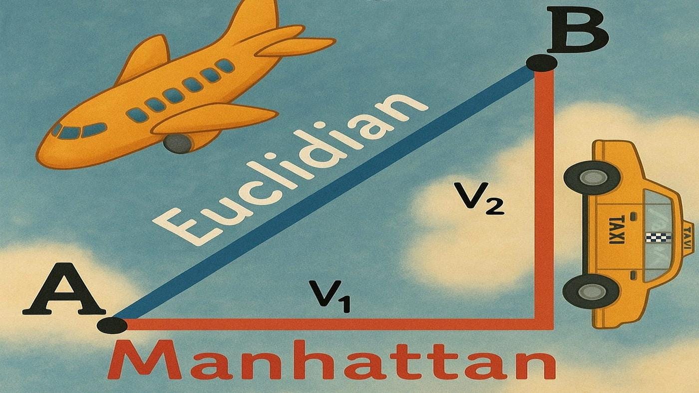
On this article we’ll journey from plain-old factors on a line all the way in which to L∞, stopping to see why L¹ and L² matter, how they differ, and the place the L∞ norm exhibits up in AI.
Our Agenda:
- When to make use of L¹ versus L² loss
- How L¹ and L² regularization pull a mannequin towards sparsity or clean shrinkage
- Why the tiniest algebraic distinction blurs GAN pictures — or leaves them razor-sharp
- generalize distance to Lᵖ house and what the L∞ norm represents
A Temporary Be aware on Mathematical Abstraction
You may need have had a dialog (maybe a complicated one) the place the time period mathematical abstraction popped up, and also you may need left that dialog feeling slightly extra confused about what mathematicians are actually doing. Abstraction refers to extracting underlying patters and properties from an idea to generalize it so it has wider software. This may appear actually sophisticated however check out this trivial instance:
A degree in 1-D is x = x₁; in 2-D: x = (x₁,x₂); in 3-D: x = (x₁, x₂, x₃). Now I don’t learn about you however I can’t visualize 42 dimensions, however the identical sample tells me a degree in 42 dimensions can be x = (x₁, …, x₄₂).
This may appear trivial however this idea of abstraction is essential to get to L∞, the place as a substitute of a degree we summary distance. Any longer let’s work with x = (x₁, x₂, x₃, …, xₙ), in any other case identified by its formal title: x∈ℝⁿ. And any vector is v = x — y = (x₁ — y₁, x₂ — y₂, …, xₙ — yₙ).
The “Regular” Norms: L1 and L2
The key takeaway is easy however highly effective: as a result of the L¹ and L² norms behave in another way in just a few essential methods, you’ll be able to mix them in a single goal to juggle two competing targets. In regularization, the L¹ and L² phrases contained in the loss perform assist strike the perfect spot on the bias-variance spectrum, yielding a mannequin that’s each correct and generalizable. In Gans, the L¹ pixel loss is paired with adversarial loss so the generator makes pictures that (i) look real looking and (ii) match the supposed output. Tiny distinctions between the 2 losses clarify why Lasso performs characteristic choice and why swapping L¹ out for L² in a GAN typically produces blurry pictures.

L¹ vs. L² Loss — Similarities and Variations

- In case your knowledge could comprise many outliers or heavy-tailed noise, you normally attain for L¹.
- When you care most about general squared error and have fairly clear knowledge, L² is okay — and simpler to optimize as a result of it’s clean.
As a result of MAE treats every error proportionally, fashions educated with L¹ sit nearer the median statement, which is precisely why L¹ loss retains texture element in GANs, whereas MSE’s quadratic penalty nudges the mannequin towards a imply worth that appears smeared.
L¹ Regularization (Lasso)
Optimization and Regularization pull in reverse instructions: optimization tries to suit the coaching set completely, whereas regularization intentionally sacrifices slightly coaching accuracy to achieve generalization. Including an L¹ penalty 𝛼∥w∥₁ promotes sparsity — many coefficients collapse all the way in which to zero. An even bigger α means harsher characteristic pruning, less complicated fashions, and fewer noise from irrelevant inputs. With Lasso, you get built-in characteristic choice as a result of the ∥w∥₁ time period actually turns small weights off, whereas L² merely shrinks them.

L2 Regularization (Ridge)
Change the regularization time period to

and you’ve got Ridge regression. Ridge shrinks weights towards zero with out normally hitting precisely zero. That daunts any single characteristic from dominating whereas nonetheless retaining each characteristic in play — useful once you imagine all inputs matter however you wish to curb overfitting.
Each Lasso and Ridge enhance generalization; with Lasso, as soon as a weight hits zero, the optimizer feels no robust purpose to go away — it’s like standing nonetheless on flat floor — so zeros naturally “stick.” Or in additional technical phrases they only mould the coefficient house in another way — Lasso’s diamond-shaped constraint set zeroes coordinates, Ridge’s spherical set merely squeezes them. Don’t fear when you didn’t perceive that, there may be various concept that’s past the scope of this text, but when it pursuits you this studying on Lₚ house ought to assist.
However again to level. Discover how after we prepare each fashions on the identical knowledge, Lasso removes some enter options by setting their coefficients precisely to zero.
from sklearn.datasets import make_regression
from sklearn.linear_model import Lasso, Ridge

X, y = make_regression(n_samples=100, n_features=30, n_informative=5, noise=10)

mannequin = Lasso(alpha=0.1).match(X, y)
print("Lasso nonzero coeffs:", (mannequin.coef_ != 0).sum())

mannequin = Ridge(alpha=0.1).match(X, y)
print("Ridge nonzero coeffs:", (mannequin.coef_ != 0).sum())
Discover how if we enhance α to 10 much more options are deleted. This may be fairly harmful as we could possibly be eliminating informative knowledge.
mannequin = Lasso(alpha=10).match(X, y)
print("Lasso nonzero coeffs:", (mannequin.coef_ != 0).sum())

mannequin = Ridge(alpha=10).match(X, y)
print("Ridge nonzero coeffs:", (mannequin.coef_ != 0).sum())
L¹ Loss in Generative Adversarial Networks (GANs)
GANs pit 2 networks towards one another, a Generator G (the “forger”) towards a Discriminator D (the “detective”). To make G produce convincing and trustworthy pictures, many image-to-image GANs use a hybrid loss

the place
- x — enter picture (e.g., a sketch)
- y— actual goal picture (e.g., a photograph)
- λ — stability knob between realism and constancy

Swap the pixel loss to L² and also you sq. pixel errors; massive residuals dominate the target, so G performs it secure by predicting the imply of all believable textures — end result: smoother, blurrier outputs. With L¹, each pixel error counts the identical, so G gravitates to the median texture patch and retains sharp boundaries.
Why tiny variations matter
- In regression, the kink in L¹’s spinoff lets Lasso zero out weak predictors, whereas Ridge solely nudges them.
- In imaginative and prescient, the linear penalty of L¹ retains high-frequency element that L² blurs away.
- In each circumstances you’ll be able to mix L¹ and L² to commerce robustness, sparsity, and clean optimization — precisely the balancing act on the coronary heart of contemporary machine-learning aims.
Generalizing Distance to Lᵖ
Earlier than we attain L∞, we have to discuss in regards to the the 4 guidelines each norm should fulfill:
- Non-negativity — A distance can’t be unfavorable; no person says “I’m –10 m from the pool.”
- Constructive definiteness — The gap is zero solely on the zero vector, the place no displacement has occurred
- Absolute homogeneity (scalability) — Scaling a vector by α scales its size by |α|: when you double your velocity you double your distance
- Triangle inequality — A detour via y isn’t shorter than going straight from begin to end (x + y)

At first of this text, the mathematical abstraction we carried out was fairly simple. However now, as we have a look at the next norms, you’ll be able to see we’re doing one thing comparable at a deeper stage. There’s a transparent sample: the exponent contained in the sum will increase by one every time, and the exponent outdoors the sum does too. We’re additionally checking whether or not this extra summary notion of distance nonetheless satisfies the core properties we talked about above. It does. So what we’ve completed is efficiently summary the idea of distance into Lᵖ house.

as a single household of distances — the Lᵖ house. Taking the restrict as p→∞ squeezes that household all the way in which to the L∞ norm.
The L∞ Norm
The L∞ norm goes by many names supremum norm, max norm, uniform norm, Chebyshev norm, however they’re all characterised by the next restrict:

By generalizing our norm to p — house, in two strains of code, we are able to write a perform that calculates distance in any norm possible. Fairly helpful.
def Lp_norm(v, p):
    return sum(abs(x)**p for x in v) ** (1/p)
We are able to now consider how our measure for distance adjustments as p will increase. Wanting on the graphs bellow we see that our measure for distance monotonically decreases and approaches a really particular level: The biggest absolute worth within the vector, represented by the dashed line in black.

In reality, it doesn’t solely method the biggest absolute coordinate of our vector however


The max-norm exhibits up any time you want a uniform assure or worst-case management. In much less technical phrases, If no particular person coordinate can transcend a sure threshold than the L∞ norm ought to be used. If you wish to set a tough cap on each coordinate of your vector then that is additionally your go to norm.
This isn’t only a quirk of concept however one thing fairly helpful, and nicely utilized in plethora of various contexts:
- Most absolute error — sure each prediction so none drifts too far.
- Max-Abs characteristic scaling — squashes every characteristic into [−1,1][-1,1][−1,1] with out distorting sparsity.
- Max-norm weight constraints — maintain all parameters inside an axis-aligned field.
- Adversarial robustness — limit every pixel perturbation to an ε-cube (an L∞ ball).
- Chebyshev distance in k-NN and grid searches — quickest technique to measure “king’s-move” steps.
- Strong regression / Chebyshev-center portfolio issues — linear packages that decrease the worst residual.
- Equity caps — restrict the biggest per-group violation, not simply the common.
- Bounding-box collision checks — wrap objects in axis-aligned packing containers for fast overlap checks.
With our extra summary notion for distance all types of fascinating questions come to the entrance. We are able to think about p worth that aren’t integers, say p = π (as you will notice within the graphs above). We are able to additionally think about p ∈ (0,1), say p = 0.3, would that also match into the 4 guidelines we mentioned each norm should obey?
Conclusion
Abstracting the concept of distance can really feel unwieldy, even needlessly theoretical, however distilling it to its core properties frees us to ask questions that may in any other case be unattainable to border. Doing so reveals new norms with concrete, real-world makes use of. It’s tempting to deal with all distance measures as interchangeable, but small algebraic variations give every norm distinct properties that form the fashions constructed on them. From the bias-variance trade-off in regression to the selection between crisp or blurry pictures in GANs, it issues the way you measure distance.
Let’s join on Linkedin!
Comply with me on X = Twitter
Code on Github


