
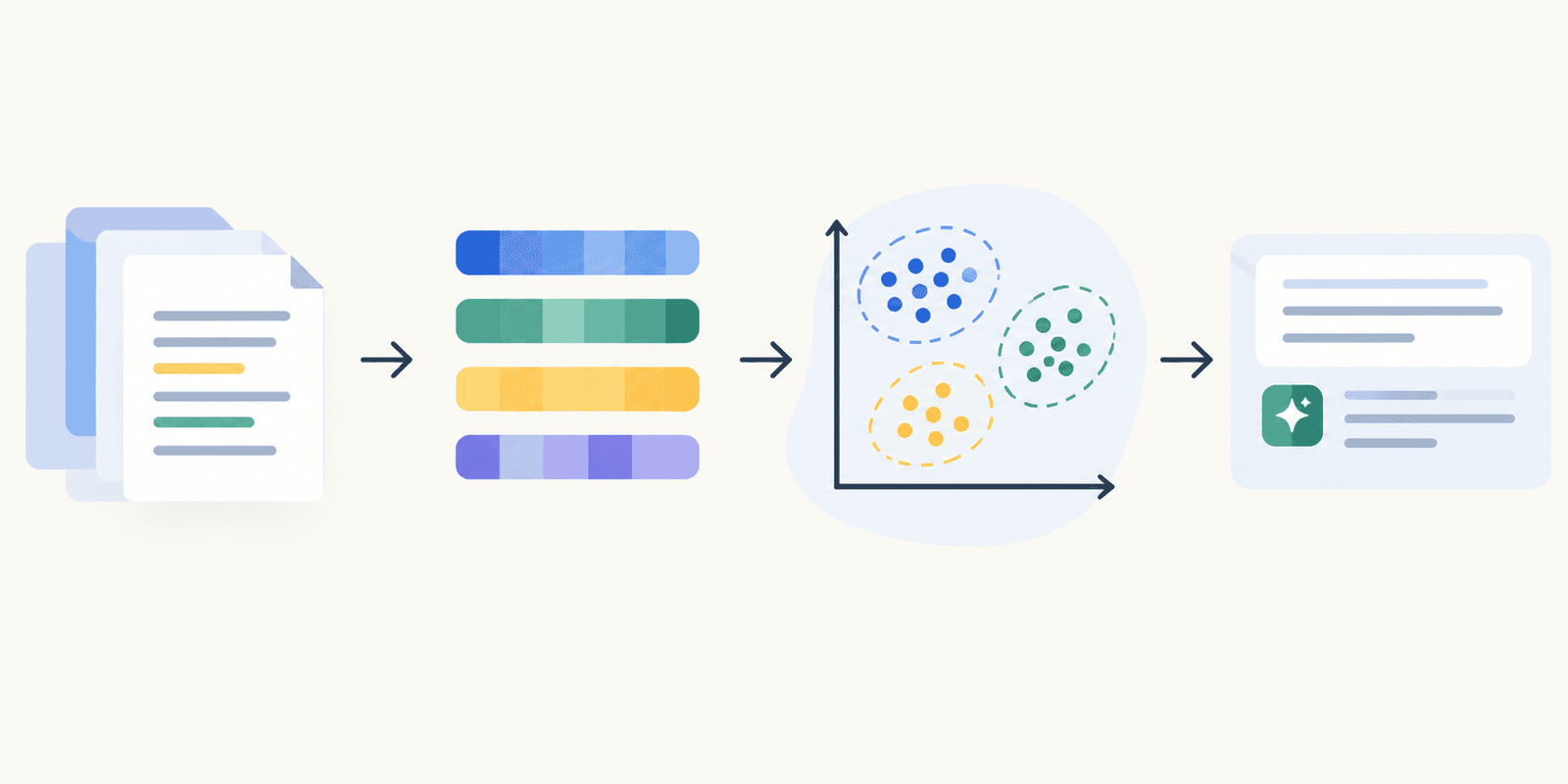
On this article, you’ll learn to construct a light-weight, end-to-end RAG pipeline utilizing scikit-learn for vector retrieval and open-source fashions for embeddings and textual content era, with out using paid APIs or heavyweight frameworks.
Subjects we are going to cowl embrace:
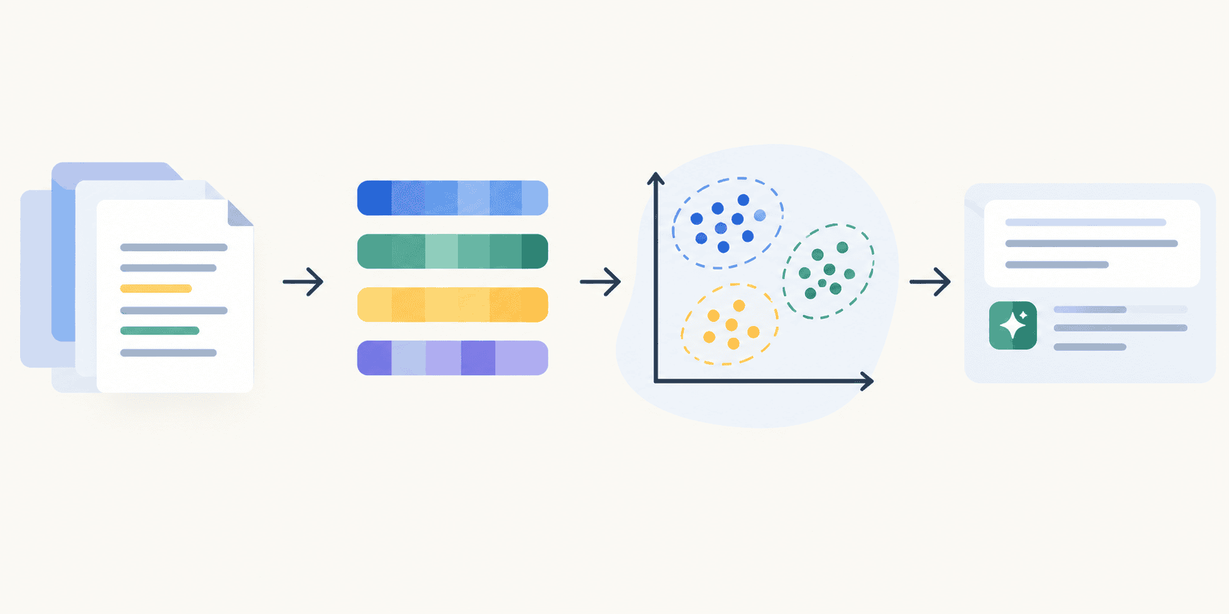
- Tips on how to obtain a doc dataset, chunk it into semantic items, and generate embeddings utilizing an area sentence-transformer mannequin.
- Tips on how to construct a customized retriever class utilizing scikit-learn’s NearestNeighbors with cosine distance as a stand-in for a vector database.
- Tips on how to wire the retriever along with a light-weight open-source LLM to provide a completely useful, in-memory RAG pipeline.
Introduction
Fashionable retrieval augmented era (RAG techniques) are sometimes regarded as inseparable from an expansive ecosystem of frameworks, together with sometimes costly, managed vector databases to retailer doc collections for retrieval.
On the core, nonetheless, RAG techniques depend on a reasonably easy notion: calculating distances between semantic vectors representing texts. It’s not strictly essential to navigate the intricacies of a devoted AI infrastructure when working with a small-to-medium-sized corpus, prototyping a brand new proof-of-concept, or deploying to environments underneath price constraints. As an alternative, we will use scikit-learn procedures along with open-source LLMs to construct clear, quick RAG pipelines that stay absolutely useful. This text exhibits how.
Step-by-Step Information
The answer supplied beneath is totally free to make use of, counting on sentence-transformers to construct native embeddings from a textual content dataset and a light-weight pre-trained LLM from Hugging Face for the era stage. If you should brush up on primary RAG ideas, take a look at this text first.
Whereas the pipeline may be carried out and run in an area IDE, for demonstration functions I like to recommend operating all the pipeline on Google Colab, utilizing its free T4 GPU for extra environment friendly execution. In case you observe this method, begin by putting in and importing the required libraries and dependencies:
|
!pip set up –q sentence–transformers transformers
import os import glob import urllib.request import zipfile import numpy as np import pandas as pd from sklearn.neighbors import NearestNeighbors from sentence_transformers import SentenceTransformer from transformers import pipeline
print(“Libraries loaded efficiently!”) |
I made obtainable a small dataset containing 9 textual content information — transient descriptions of Asian nations — in a public GitHub repository. You possibly can obtain it, extract the information, and save the texts in a easy record as follows:
|
1 2 3 4 5 6 7 8 9 10 11 12 13 14 15 16 17 |
# Downloading and extracting the toy dataset, containing 9 paperwork url = “https://github.com/gakudo-ai/open-datasets/blob/essential/asia_documents.zip?uncooked=true” zip_path = “asia_documents.zip” extract_dir = “asia_documents”
urllib.request.urlretrieve(url, zip_path) with zipfile.ZipFile(zip_path, ‘r’) as zip_ref: zip_ref.extractall(extract_dir)
# Studying all extracted textual content information paperwork = [] for filepath in glob.glob(f“{extract_dir}/**/*.txt”, recursive=True): with open(filepath, ‘r’, encoding=‘utf-8’) as file: paperwork.append(file.learn())
print(f“Loaded {len(paperwork)} paperwork.”) # If the zip contained a CSV as an alternative, you’d use pd.read_csv() right here. |
The dataset we simply loaded will represent our miniature doc base for RAG. We have to put it in the precise format — that’s, flip the texts into embedding vectors. Earlier than doing that, it is not uncommon apply in RAG to chunk paperwork into smaller, semantic items that the embedding mannequin — answerable for mapping items of textual content into numerical embeddings — can course of extra successfully. The texts in our dataset don’t actually require chunking as a result of they’re fairly brief, however we’re simulating this step as an example greatest practices in real-world RAG pipelines.
We outline a local chunking perform, utilizing smaller-than-usual values for chunk dimension and overlap (each measured in phrases) in order that we will observe some precise impact on our small paperwork:
|
def chunk_text(textual content, chunk_size=25, overlap=5): “”“Splits textual content into chunks natively, with out exterior frameworks.”“” phrases = textual content.break up() chunks = [] for i in vary(0, len(phrases), chunk_size – overlap): chunk = ” “.be part of(phrases[i:i + chunk_size]) chunks.append(chunk) return chunks
# Processing all paperwork right into a flat record of chunks all_chunks = [] for doc in paperwork: all_chunks.lengthen(chunk_text(doc))
print(f“Created {len(all_chunks)} chunks from the unique paperwork.”) |
Output:
|
Created 31 chunks from the authentic paperwork. |
In a real-world utility, you’ll possible use considerably bigger values for each arguments within the chunking perform.
Subsequent, we generate the embeddings utilizing a preferred light-weight mannequin for this job: the 'all-MiniLM-L6-v2' sentence-transformer:
|
# Initializing the embedding mannequin (runs regionally on Colab’s free CPU/GPU) embedding_model = SentenceTransformer(‘all-MiniLM-L6-v2’)
# Producing embeddings for all textual content chunks print(“Producing embeddings… (that is quick on Colab!)”) chunk_embeddings = embedding_model.encode(all_chunks, show_progress_bar=True) |
As soon as we’ve a group of embeddings, it’s time to outline one of many key elements of any RAG pipeline: the retriever. Since we’re doing this the scikit-learn approach, we are going to wrap sklearn.neighbors.NearestNeighbors — a easy but efficient distance calculation algorithm — right into a clear, reusable class that mimics the performance of a vector database, all based mostly on cosine distance, which is right for embedding vector representations.
|
1 2 3 4 5 6 7 8 9 10 11 12 13 14 15 16 17 18 19 20 21 22 23 |
class SklearnRetriever: def __init__(self, n_neighbors=3): # Utilizing ‘cosine’ metric as a result of LLM embeddings measure semantic similarity based mostly on angles between vectors self.retriever = NearestNeighbors(n_neighbors=n_neighbors, metric=‘cosine’, algorithm=‘brute’) self.chunks = []
def match(self, chunks, embeddings): “”“Indexes the paperwork.”“” self.chunks = chunks self.retriever.match(embeddings) print(“Vector index constructed efficiently!”)
def retrieve(self, query_embedding): “”“Returns probably the most related chunks for a given question.”“” distances, indices = self.retriever.kneighbors([query_embedding])
# Fetching the precise textual content strings utilizing the retrieved indices outcomes = [self.chunks[idx] for idx in indices[0]] return outcomes
# Instantiating and becoming our customized retriever vector_db = SklearnRetriever(n_neighbors=3) vector_db.match(all_chunks, chunk_embeddings) |
The opposite main element of the pipeline is the generator. Right here too we hold issues light-weight, selecting a small, open-source LLM educated for pure language era: Qwen/Qwen2.5-0.5B-Instruct. This mannequin is sufficiently small to run easily on a Colab pocket book with out risking a RAM crash.
|
1 2 3 4 5 6 7 8 9 10 11 12 13 14 15 16 17 18 19 20 21 22 |
# Loading a light-weight causal LLM constructed for the “text-generation” pipeline llm = pipeline(“text-generation”, mannequin=“Qwen/Qwen2.5-0.5B-Instruct”, device_map=“auto”)
def generate_rag_answer(question, retrieved_context): “”“Combines the immediate, context, and question for the LLM utilizing chat formatting.”“” context_str = ” — “.be part of(retrieved_context)
messages = [ {“role”: “system”, “content”: “You are a helpful assistant. Answer the user’s question using ONLY the provided context. If the answer is not in the context, say ‘I cannot find the answer in the provided documents.'”}, {“role”: “user”, “content”: f“Context:n{context_str}nnQuestion: {query}”} ]
# Apply the mannequin’s chat template immediate = llm.tokenizer.apply_chat_template(messages, tokenize=False, add_generation_prompt=True)
# Producing the response response = llm(immediate, max_new_tokens=150, do_sample=False, temperature=0.1)
# Extracting solely the newly generated textual content previous the immediate generated_text = response[0][‘generated_text’] reply = generated_text[len(prompt):].strip() return reply |
All of the items of the pipeline at the moment are in place. The final step is to wire them collectively and attempt it out by asking our system a query about its data base (Asian nations):
|
1 2 3 4 5 6 7 8 9 10 11 12 13 14 15 16 17 18 19 20 |
def ask_rag_pipeline(query): print(f“Query: {query}”)
# 1. Embedding the question query_vector = embedding_model.encode(query)
# 2. Retrieving context through Scikit-Be taught relevant_chunks = vector_db.retrieve(query_vector)
# 3. Producing Reply reply = generate_rag_answer(query, relevant_chunks)
print(f“nRAG Reply: {reply}”) print(“n— Sources used —“) for i, chunk in enumerate(relevant_chunks): print(f“{i+1}. {chunk[:100]}…”) # Truncated for readability
# Testing it out test_question = “Which Asian nations are greatest identified for islands and seashores?” ask_rag_pipeline(test_question) |
Output:
|
Query: Which Asian nations are greatest identified for islands and seashores?
RAG Reply: The Asian nations that are greatest identified for islands and seashores embrace:
1. Philippines – Identified for its over 7,000 islands and vibrant festivals. 2. Thailand – Well-known for its tropical seashores and bustling road meals tradition.
These two nations have a important quantity of islands and provide each lovely pure surroundings and various seaside experiences.
—– Sources used —– 1. mountainous landscapes and cultural cities like Chiang Mai, whereas the south gives world–famend is... 2. The Philippines is an archipelago of over 7,000 islands in Southeast Asia, identified for its gorgeous be... 3. Thailand is a Southeast Asian nation well-known for its tropical seashores, ornate temples, and bustling ... |
Strive asking totally different questions by changing the textual content in test_question. The habits and outputs are affordable given the small-scale setup we simply constructed — although don’t count on industrial LLM-level outcomes: we’re combining a small mannequin with a tiny data base.
Last Remarks
On this article, we constructed a light-weight, end-to-end RAG pipeline that avoids the overhead of heavyweight frameworks or paid APIs. It depends solely on scikit-learn vector retrieval and open-source fashions for each embeddings and era, producing a clear, in-memory system. This method makes a stable place to begin for prototyping, experimenting with totally different retrieval methods, and validating ideas earlier than scaling up.