we’re.
That is the mannequin that motivated me, from the very starting, to make use of Excel to raised perceive Machine Studying.
And at present, you’ll see a totally different rationalization of SVM than you normally see, which is the one with:
- margin separators,
- distances to a hyperplane,
- geometric constructions first.
As a substitute, we are going to construct the mannequin step-by-step, ranging from issues we already know.
So perhaps that is additionally the day you lastly say “oh, I perceive higher now.”
Constructing a New Mannequin on What We already Know
One among my foremost studying ideas is easy:
at all times begin from what we already know.
Earlier than SVM, we already studied:
- logistic regression,
- penalization and regularization.
We are going to use these fashions and ideas at present.
The thought is to not introduce a brand new mannequin, however to rework an present one.
Coaching datasets and label conference
We are going to use a one-feature dataset to clarify the SVM.
Sure, I do know, that is most likely the primary time you see somebody clarify SVM utilizing just one characteristic.
Why not?
In actual fact, it’s vital, for a number of causes.
For different fashions, akin to linear regression or logistic regression, we normally begin with a single characteristic. We must always do the identical with SVM, in order that we are able to examine the fashions correctly.
Should you construct a mannequin with many options and assume you perceive the way it works, however you can not clarify it with only one characteristic, then you don’t actually perceive it but.
Utilizing a single characteristic makes the mannequin:
- less complicated to implement,
- simpler to visualise,
- and far simpler to debug.
So, we use two datasets that I generated for example the 2 attainable conditions a linear classifier can face:
- one dataset is fully separable
- the opposite is not fully separable
It’s possible you’ll already know why we use these two datasets, whereas we solely use one, proper?
We additionally use the label conference -1 and 1 as an alternative of 0 and 1.
Why? We are going to see later, that’s truly fascinating historical past, about how the fashions are seen in GLM and Machine Studying views.

In logistic regression, earlier than making use of the sigmoid, we compute a logit. And we are able to name it f, this can be a linear rating.
This amount is a linear rating that may take any actual worth, from −∞ to +∞.
- optimistic values correspond to at least one class,
- adverse values correspond to the opposite,
- zero is the choice boundary.
Utilizing labels -1 and 1 matches this interpretation naturally.
It emphasizes the signal of the logit, with out going via possibilities.
So, we’re working with a pure linear mannequin, not inside the GLM framework.
There is no such thing as a sigmoid, no likelihood, solely a linear choice rating.
A compact option to specific this concept is to take a look at the amount:
y(ax + b) = y f(x)
- If this worth is optimistic, the purpose is accurately categorised.
- Whether it is giant, the classification is assured.
- Whether it is adverse, the purpose is misclassified.
At this level, we’re nonetheless not speaking about SVMs.
We’re solely making specific what good classification means in a linear setting.
From log-loss to a brand new loss perform
With this conference, we are able to write the log-loss for logistic regression instantly as a perform of the amount:
y f(x) = y (ax+b)
We will plot this loss as a perform of yf(x).
Now, allow us to introduce a brand new loss perform known as the hinge loss.
After we plot the 2 losses on the identical graph, we are able to see that they’re fairly comparable in form.
Do you keep in mind Gini vs. Entropy in Choice Tree Classifiers?
The comparability may be very comparable right here.

In each circumstances, the thought is to penalize:
- factors which might be misclassified yf(x)<0,
- factors which might be too near the choice boundary.
The distinction is in how this penalty is utilized.
- The log-loss penalizes errors in a clean and progressive approach.
Even well-classified factors are nonetheless barely penalized. - The hinge loss is extra direct and abrupt.
As soon as some extent is accurately categorised with a ample margin, it’s now not penalized in any respect.
So the purpose is to not change what we take into account a great or unhealthy classification,
however to simplify the way in which we penalize it.
One query naturally follows.
May we additionally use a squared loss?
In spite of everything, linear regression will also be used as a classifier.
However after we do that, we instantly see the issue:
the squared loss retains penalizing factors which might be already very nicely categorised.
As a substitute of specializing in the choice boundary, the mannequin tries to suit precise numeric targets.
For this reason linear regression is normally a poor classifier, and why the selection of the loss perform issues a lot.

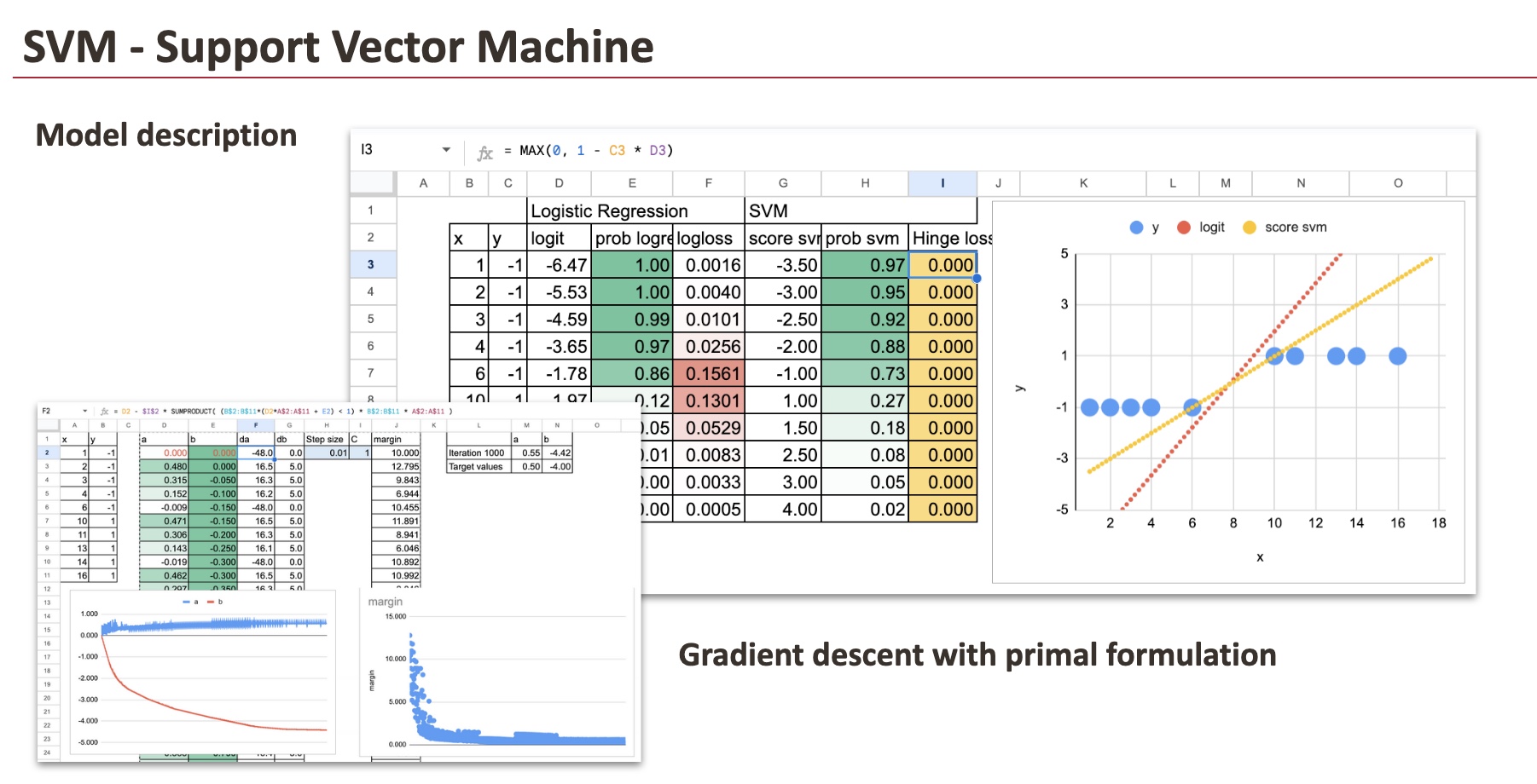
Description of the brand new mannequin
Allow us to now assume that the mannequin is already skilled and look instantly on the outcomes.
For each fashions, we compute precisely the identical portions:
- the linear rating (and it’s known as logit for Logistic Regression)
- the likelihood (we are able to simply apply the sigmoid perform in each circumstances),
- and the loss worth.
This enables a direct, point-by-point comparability between the 2 approaches.
Though the loss capabilities are totally different, the linear scores and the ensuing classifications are very comparable on this dataset.
For the fully separable dataset, the result’s rapid: all factors are accurately categorised and lie sufficiently removed from the choice boundary. As a consequence, the hinge loss is the same as zero for each remark.
This results in an vital conclusion.
When the information is completely separable, there may be not a novel resolution. In actual fact, there are infinitely many linear choice capabilities that obtain precisely the identical end result. We will shift the road, rotate it barely, or rescale the coefficients, and the classification stays good, with zero loss all over the place.
So what can we do subsequent?
We introduce regularization.
Simply as in ridge regression, we add a penalty on the measurement of the coefficients. This extra time period doesn’t enhance classification accuracy, however it permits us to pick out one resolution amongst all of the attainable ones.
So in our dataset, we get the one with the smallest slope a.

And congratulations, we now have simply constructed the SVM mannequin.
We will now simply write down the fee perform of the 2 fashions: Logistic Regression and SVM.
Do you keep in mind that Logistic Regression might be regularized, and it’s nonetheless known as so, proper?

Now, why does the mannequin embrace the time period “Help Vectors”?
Should you take a look at the dataset, you’ll be able to see that just a few factors, for instance those with values 6 and 10, are sufficient to find out the choice boundary. These factors are known as assist vectors.
At this stage, with the angle we’re utilizing, we can not establish them instantly.
We are going to see later that one other viewpoint makes them seem naturally.
And we are able to do the identical train for one more dataset, with non-separable dataset, however the precept is identical. Nothing modified.
However now, we are able to see that for certains factors, the hinge loss shouldn’t be zero. In our case beneath, we are able to see visually that there are 4 factors that we’d like as Help Vectors.

SVM Mannequin Coaching with Gradient Descent
We now prepare the SVM mannequin explicitly, utilizing gradient descent.
Nothing new is launched right here. We reuse the identical optimization logic we already utilized to linear and logistic regression.
New conference: Lambda (λ) or C
In lots of fashions we studied beforehand, akin to ridge or logistic regression, the target perform is written as:
data-fit loss +λ ∥w∥
Right here, the regularization parameter λ controls the penalty on the scale of the coefficients.
For SVMs, the standard conference is barely totally different. We moderately use C in entrance of the data-fit time period.

Each formulations are equal.
They solely differ by a rescaling of the target perform.
We hold the parameter C as a result of it’s the usual notation utilized in SVMs. And we are going to see why we now have this conference later.
Gradient (subgradient)
We work with a linear choice perform, and we are able to outline the margin for every level as: mi = yi (axi + b)
Solely observations such that mi<1 contribute to the hinge loss.
The subgradients of the target are as follows, and we are able to implement in Excel, utilizing logical masks and SUMPRODUCT.

Parameter replace
With a studying price or step measurement η, the gradient descent updates are as follows, and we are able to do the standard method:

We iterate these updates till convergence.
And, by the way in which, this coaching process additionally provides us one thing very good to visualise. At every iteration, because the coefficients are up to date, the measurement of the margin adjustments.
So we are able to visualize, step-by-step, how the margin evolves throughout the studying course of.
Optimization vs. geometric formulation of SVM
This determine beneath exhibits the similar goal perform of the SVM mannequin written in two totally different languages.

On the left, the mannequin is expressed as an optimization drawback.
We reduce a mix of two issues:
- a time period that retains the mannequin easy, by penalizing giant coefficients,
- and a time period that penalizes classification errors or margin violations.
That is the view we now have been utilizing to date. It’s pure after we assume by way of loss capabilities, regularization, and gradient descent. It’s the most handy kind for implementation and optimization.
On the suitable, the identical mannequin is expressed in a geometric approach.
As a substitute of speaking about losses, we speak about:
- margins,
- constraints,
- and distances to the separating boundary.
When the information is completely separable, the mannequin seems to be for the separating line with the largest attainable margin, with out permitting any violation. That is the hard-margin case.
When good separation is not possible, violations are allowed, however they’re penalized. This results in the soft-margin case.
What’s vital to know is that these two views are strictly equal.
The optimization formulation mechanically enforces the geometric constraints:
- penalizing giant coefficients corresponds to maximizing the margin,
- penalizing hinge violations corresponds to permitting, however controlling, margin violations.
So this isn’t two totally different fashions, and never two totally different concepts.
It’s the similar SVM, seen from two complementary views.
As soon as this equivalence is evident, the SVM turns into a lot much less mysterious: it’s merely a linear mannequin with a selected approach of measuring errors and controlling complexity, which naturally results in the maximum-margin interpretation everybody is aware of.
Unified Linear Classifier
From the optimization viewpoint, we are able to now take a step again and take a look at the larger image.
What we now have constructed isn’t just “the SVM”, however a common linear classification framework.
A linear classifier is outlined by three unbiased decisions:
- a linear choice perform,
- a loss perform,
- a regularization time period.
As soon as that is clear, many fashions seem as easy combos of those components.
In observe, that is precisely what we are able to do with SGDClassifier in scikit-learn.

From the identical viewpoint, we are able to:
- mix the hinge loss with L1 regularization,
- change hinge loss with squared hinge loss,
- use log-loss, hinge loss, or different margin-based losses,
- select L2 or L1 penalties relying on the specified habits.
Every selection adjustments how errors are penalized or how coefficients are managed, however the underlying mannequin stays the identical: a linear choice perform skilled by optimization.
Primal vs Twin Formulation
It’s possible you’ll have already got heard in regards to the twin kind of SVM.
Up to now, we now have labored fully within the primal kind:
- we optimized the mannequin coefficients instantly,
- utilizing loss capabilities and regularization.
The twin kind is one other option to write the identical optimization drawback.
As a substitute of assigning weights to options, the twin kind assigns a coefficient, normally known as alpha, to every knowledge level.
We won’t derive or implement the twin kind in Excel, however we are able to nonetheless observe its end result.
Utilizing scikit-learn, we are able to compute the alpha values and confirm that:
- the primal and twin types result in the similar mannequin,
- similar choice boundary, similar predictions.

What makes the twin kind notably fascinating for SVM is that:
- most alpha values are precisely zero,
- just a few knowledge factors have non-zero alpha.
These factors are the assist vectors.
This habits is particular to margin-based losses just like the hinge loss.
Lastly, the twin kind additionally explains why SVMs can use the kernel trick.
By working with similarities between knowledge factors, we are able to construct non-linear classifiers with out altering the optimization framework.
We are going to see this tomorrow.
Conclusion
On this article, we didn’t method SVM as a geometrical object with sophisticated formulation. As a substitute, we constructed it step-by-step, ranging from fashions we already know.
By altering solely the loss perform, then including regularization, we naturally arrived on the SVM. The mannequin didn’t change. Solely the way in which we penalize errors did.
Seen this fashion, SVM shouldn’t be a brand new household of fashions. It’s a pure extension of linear and logistic regression, seen via a distinct loss.
We additionally confirmed that:
- the optimization view and the geometric view are equal,
- the maximum-margin interpretation comes instantly from regularization,
- and the notion of assist vectors emerges naturally from the twin perspective.
As soon as these hyperlinks are clear, SVM turns into a lot simpler to know and to put amongst different linear classifiers.
Within the subsequent step, we are going to use this new perspective to go additional, and see how kernels lengthen this concept past linear fashions.


