Optimizing Deep Studying Fashions with SAM

: Overparameterization, Generalizability, and SAM

The dramatic success of contemporary deep studying — particularly within the domains of Pc Imaginative and prescient and Pure Language Processing — is constructed on “overparameterized” fashions: fashions with greater than sufficient parameters to memorize the coaching information completely. Functionally, a mannequin will be recognized as overparameterized when it may possibly simply obtain a near-perfect coaching accuracy (near 100%) with near-zero coaching loss for a given activity.

Nevertheless, the usefulness of such a mannequin depends upon whether or not it performs properly on the held-out check information drawn from the identical distribution because the coaching set, however unseen throughout coaching. This property is named “generalizability” — the flexibility of a mannequin to take care of efficiency on new examples — and it’s important for any deep studying mannequin to be virtually helpful.

Classical Machine Studying concept tells us that overparameterized fashions ought to catastrophically overfit and subsequently generalize poorly. Nevertheless, one of the crucial stunning discoveries of the previous decade is that fashions on this class usually generalize remarkably properly.

This extremely counterintuitive phenomenon has been investigated in a sequence of papers, beginning with the seminal works of Belkin et al. (2018) and Nakkiran et al. (2019), which demonstrated that there exists a “double descent” curve for generalizability: as mannequin measurement will increase, generalization first worsens (as classical concept predicts), then improves once more past a important threshold — supplied the mannequin is educated with the suitable optimization strategies.

Determine 1 exhibits a cartoon of a double descent curve. The y-axis plots check error — a measure of generalizability, the place decrease error signifies higher generalization — whereas the x-axis exhibits the variety of mannequin parameters. As mannequin measurement will increase, coaching error (dashed blue line) quickly approaches zero, as anticipated.

The check error (stable blue line) displays a extra attention-grabbing habits: it initially decreases with mannequin measurement — the primary descent, highlighted by the left purple circle — after which rises to a peak on the interpolation threshold marked by the vertical dashed line, the place the mannequin has the worst generalization. Past this threshold, nonetheless, within the overparameterized regime, the check error decreases once more — the second descent, highlighted by the best purple circle — and continues to say no as extra parameters are added. That is the regime of curiosity for contemporary deep studying fashions. 

In Machine Studying, one finds the parameters of a mannequin by minimizing a loss perform on the coaching dataset. However does merely minimizing our favourite loss perform — like cross-entropy — on the coaching dataset assure passable generalization properties for the category of overparametrized fashions? The reply is — usually talking — no! Whether or not one is concerned about fine-tuning a pre-trained mannequin or coaching a mannequin from scratch, you will need to optimize your coaching algorithm to make sure that you may have a sufficiently generalizable mannequin. That is what makes the selection of the optimizer a vital design alternative.

Sharpness-Conscious-Minimization (SAM) — launched in a paper by Foret et al. (2019) — is an optimizer designed to enhance generalizability of an overparameterized mannequin. On this article, I current a pedagogical evaluate of SAM that features:

1. An intuitive understanding of how SAM works and why it improves generalization.
2. A deep dive into the algorithm, explaining the important thing mathematical steps concerned. 
3. A PyTorch implementation of the optimizer class in a coaching loop, together with an vital caveat for fashions with BatchNorm layers.
4. A fast demonstration of the effectiveness of the optimizer in enhancing generalization on a picture classification activity with a ResNet-18 mannequin.

The entire code used on this article will be present in this Github repo — be at liberty to mess around with it!

The Notion of Sharpness

To start with, allow us to attempt to get an intuitive sense of why merely minimizing the loss perform is probably not sufficient for optimum generalization. 

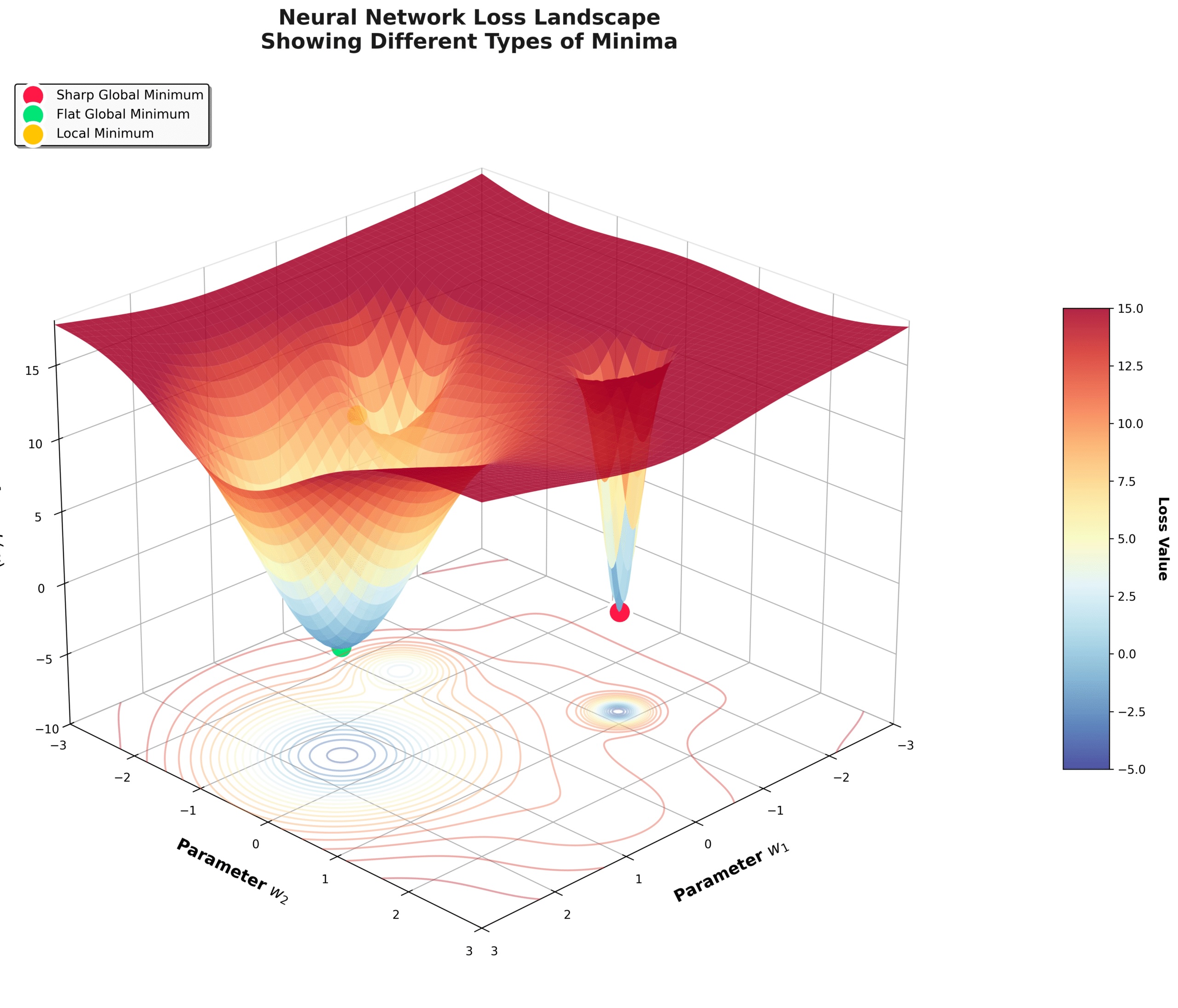
A helpful image to take note of is that of the loss panorama. For a big overparametrized mannequin, the loss panorama has a number of native and world minima. The native geometries round such minima can range considerably alongside the panorama. For instance, two minima might have practically similar loss values, but differ dramatically of their native geometry: one could also be sharp (slender valley) whereas the opposite is flat (huge valley).

One formal measure for evaluating these native geometries is “sharpness”. At any given level w within the loss panorama with loss perform L(w), sharpness S(w) is outlined as:

Let me unpack the definition. Think about you’re at a degree w within the loss panorama and also you perturb the parameters such that the brand new parameter at all times lies inside a ball of radius ρ with middle w. Sharpness is then outlined because the maximal change within the loss perform inside this household of perturbations. Within the literature, additionally it is known as the worst-direction sharpness for apparent causes.

One can readily see that for a pointy minimal — a steep, slender valley — the worth of the loss perform will change dramatically with small perturbations in sure instructions and result in a excessive worth for sharpness. For a flat minimal alternatively — a large valley — the worth of loss perform will change comparatively slowly with small perturbations and result in a decrease worth for sharpness. Subsequently, sharpness provides a measure of flatness for a given minimal within the loss panorama. 

There exists a deep connection between the native geometry of a minimal — particularly the sharpness measure— and the generalization property of the resultant mannequin. During the last decade, a major quantity of theoretical and empirical analysis has gone into clarifying this connection. As an example — because the paper by Keskar et al. (2016) factors out — world minima with related values of the loss perform can have considerably completely different generalization properties relying on their sharpness measures.

The essential lesson that appears to be emerge from these research is: flatter (much less sharp) minima are positively correlated with higher generalization of fashions. Specifically, the mannequin ought to keep away from getting caught in a pointy minima throughout coaching if it has to generalize properly. Subsequently, for coaching a mannequin with good generalization, one must be certain that the optimization process not solely minimizes the loss perform but additionally seeks to maximise the flatness (or equivalently reduce the sharpness) of the minima. 

That is exactly the issue that the SAM optimizer is designed to unravel, and that is what we flip to within the subsequent part. 

A fast apart: word that the above image provides a conceptual clarification of why an overparameterized mannequin can doubtlessly keep away from the issue of overfitting. It’s as a result of a big mannequin has a wealthy loss panorama which supplies a multiplicity of flat world minima with wonderful generalization properties.

The Sharpness-Conscious Minimization (SAM) Algorithm

Allow us to recall the usual optimization of a mannequin. It entails discovering mannequin parameters that reduce a given loss perform computed over a mini-batch B. At each time-step, one computes the gradient of the loss with respect to the parameters, and updates the parameters in response to the rule: 

In contrast to SGD or Adam, SAM doesn’t reduce L straight. As a substitute, at a given level within the loss panorama, it first scans its neighborhood of a given measurement ρ and finds the perturbation that maximizes the loss perform. Within the second step, it minimizes this most loss perform. This permits the optimizer to search out parameters that lie in neighborhoods with uniformly low loss worth, which leads to smaller sharpness values and flatter minima.

Let’s focus on the process in somewhat extra element. The loss perform for the SAM optimizer is:

the place ρ denotes the higher sure on the scale of the perturbations. The perturbation that maximizes the perform L (usually known as adversarial perturbation because it maximizes the standard loss) will be discovered by noting that:

the place the second equality is an approximation obtained by Taylor-expanding the perturbed perform in step one, and the final equality follows from the ϵ-independence of the primary time period in sq. brackets within the earlier step. This final equality will be solved for the adversarial perturbation as follows:

Plugging this again within the equation for the SAM loss, one can compute the gradients of the SAM loss to the main order in derivatives of ϵ:

That is essentially the most essential equation for the optimization process. To the main order in derivatives of ϵ, the gradients of the SAM loss perform will be approximated by the gradients of the standard loss perform evaluated on the adversarially perturbed level. Utilizing the above components for the gradients, one can now execute the usual optimizer step:

This completes one full SAM iteration. Subsequent, allow us to translate the algorithm from English to PyTorch.

PyTorch Implementation in a Coaching Loop

An illustrative instance of a coaching loop with a SAM optimizer is given within the code block sam_training_loop.py. For concreteness, we now have chosen a generic picture classification downside, however the identical construction broadly holds for a variety of Pc Imaginative and prescient and NLP duties. The SAM optimizer class is proven within the code block sam_optimizer_class.py.

Be aware that defining a SAM optimizer requires specifying two items of knowledge:

1. A base optimizer (like SGD or Adam), since SAM entails an ordinary optimizer step ultimately.
2. A hyperparameter ρ, which places an higher sure on the scale of the admissible perturbations.

A single iteration of the optimizer entails two ahead passes and two backward passes. Let’s hint out the important thing steps of the code in sam_training_loop.py:

1. Line 5 computes the loss perform L(w, B) for the present mini-batch B — the primary ahead go.
2. Line 6 computes the gradients of the loss perform L(w, B) — the primary backward go. 
3. Line 7 calls the perform sam_optimizer.first_step from the SAM optimizer class (see under) that computes the adversarial perturbation utilizing the components mentioned above, and perturbs the weights of the mannequin as mentioned earlier than.
4. Line 10 computes the loss perform for the perturbed mannequin — the second ahead go. 
5. Line 11 computes the gradients of the loss perform for the perturbed mannequin— the second backward go. 
6. Line 12 calls the perform sam_optimizer.second_step from the optimizer class (see under) that restores the weights to w_t after which makes use of the bottom optimizer to replace the weights w_t utilizing the gradients computed on the perturbed level. 

A Caveat: SAM with BatchNorm

There is a vital level that one wants to bear in mind whereas deploying SAM in a coaching loop if the mannequin has any module that features batch-normalization layers. Throughout coaching, BatchNorm implements the normalization utilizing the present batch statistics and updates the working statistics at each ahead go. For analysis, it makes use of the working statistics. 

Now, as we noticed above, SAM entails two ahead passes per iteration. For the primary go, BatchNorm works in the usual vogue. Through the second go, nonetheless, we’re utilizing perturbed weights to compute loss, and the naive coaching perform within the code block sam_training_loop.py will permit the BatchNorm layers to replace the working statistics throughout the second go as properly. That is undesirable as a result of the working statistics ought to solely mirror the habits of the unique mannequin, not the perturbed mannequin which is just an intermediate step for computing gradients. Subsequently, one has to explicitly disable the working statistics replace throughout the second go and allow it earlier than the following iteration.

For this function, we’ll use two express features disable_bn_stats and enable_bn_stats within the coaching loop — easy examples of such features are proven in code block running_stat.py — they toggle the track_running_stats parameter (line 4 and line 9) of BatchNorm perform in PyTorch. The modified coaching loop is given within the code block mod_train.py. 

Demo: Picture classification with ResNet-18

Lastly, let’s exhibit how the SAM optimization improves the generalization of a mannequin in a concrete instance. We are going to think about a picture classification downside utilizing the Style-MNIST dataset (MIT License): it consists of 60,000 coaching photos and 10,000 testing photos throughout 10 distinct, mutually unique lessons, the place every picture is grayscale with 28*28 pixels.

Because the classifier mannequin, we’ll select a PreAct ResNet-18 with none pre-training. Whereas a dialogue on the exact ResNet-18 structure just isn’t very related for our function, allow us to recall that the mannequin consists of a sequence of constructing blocks, every of which is made up of convolutional layers, BatchNorm layers, ReLU activation with skipped connections. The PreAct (pre-activation) signifies that the activation perform (ReLU) comes earlier than the convolutional layer in every block. For the standard ResNet-18, it’s the different manner spherical. I might refer the reader to the paper — He et al. (2015) — for extra particulars on the structure.

What’s vital to notice, nonetheless, is that this mannequin has about 11.2 million parameters, and subsequently from the angle of classical Machine Studying, it’s an overparameterized mannequin with the parameter-to-sample ratio being about 186:1. Additionally, for the reason that mannequin contains BatchNorm layers, we now have to watch out about disabling the working statistics for the second go, whereas utilizing SAM.

We at the moment are prepared to hold out the next experiment. We practice the mannequin on the Style-MNIST dataset with the usual SGD optimizer first after which with the SAM optimizer utilizing the identical SGD as the bottom optimizer. We are going to think about a easy setup with a set studying fee lr=0.05 and with the momentum and the weight-decay each set to zero. The hyperparameter ρ in SAM is about to 0.05. All runs are carried out on a single A100 GPU. 

Since every SAM weight replace requires two backpropagation steps — one to compute the perturbations and one other to compute the ultimate gradients — for a good comparability every non-SAM coaching run should execute twice as many epochs as every SAM coaching run. We are going to subsequently have to check a metric from one epoch of SAM coaching run to a metric from two epochs of non-SAM coaching run. We are going to name this a “standardized epoch” and a metric recorded at standardized epochs will probably be labelled as metric_st. We are going to limit the experiment to 150 standardized epochs, which suggests the SAM coaching runs for 150 epochs and the non-SAM coaching runs for 300 epochs. We are going to practice the SAM-optimized mannequin for an extra 50 epochs to get an thought of how the mannequin behaves on longer coaching. 

In making an attempt to test which optimizer provides higher generalization, we’ll examine the next two metrics after every standardized epoch of coaching:

1. Check accuracy: Efficiency of the mannequin on the check dataset.
2. Generalizability hole: Distinction between the coaching accuracy and check accuracy.

The check accuracy is an absolute measure of how properly the mannequin generalizes after a sure variety of coaching epochs. The generalizability hole, alternatively, is a diagnostic that tells you ways a lot a mannequin is overfitting at a given stage of coaching. 

Allow us to start by evaluating the training_loss_st and training_accuracy_st graphs, as proven in Determine 3. The mannequin with SGD reaches near-zero loss and near 99% coaching accuracy inside 150 epochs, as anticipated of an overparametrized mannequin. It’s evident that SAM trains slowly in comparison with SGD and takes extra standardized epochs to achieve a near-perfect coaching accuracy. That is evident from the truth that the coaching loss in addition to the coaching accuracy continues to enhance as one trains the SAM-optimized mannequin for extra epochs past the stipulated 150.

Check accuracy. The graphs in Determine 4 compares the check accuracies for the 2 circumstances after every standardized epoch.

The SGD-optimized mannequin reaches 92% check accuracy round epoch 50 and plateaus round that worth for the following 100 epochs. The SAM-optimized mannequin generalizes poorly within the preliminary part of the coaching — till round 80 epochs — as evident from the decrease check accuracies on this part in comparison with the SGD graph. Nevertheless, round epoch 80, it catches up with the SGD graph and finally surpasses it by a skinny margin.

For this particular run, on the finish of 150 epochs, the check accuracy for SAM stands at test_SAM = 92.5%, whereas that for SGD is test_SGD = 92.0%. Be aware that that is even supposing the SAM-trained mannequin has a a lot decrease coaching accuracy and coaching loss at this stage. If one trains the SAM-model for an additional 50 epochs, the check accuracy improves barely to 92.7%.

Generalization Hole. The evolution of the generalization hole after every standardized epoch in course of the coaching course of is proven in Determine 5.

The hole for the SGD mannequin grows steadily with coaching and after 150 epochs reaches gap_SGD=6.8%, whereas for SAM it grows way more slowly and reaches gap_SAM= 2.3%. On additional coaching for an additional 50 epochs, the hole for SAM climbs to round 3%, however it’s nonetheless a lot decrease in comparison with the SGD worth.

Whereas the distinction in check accuracies is small between the 2 optimizers for the Style-MNIST dataset, there’s a non-trivial distinction within the generalization gaps, which demonstrates that optimizing with SAM results in higher generalization.

Concluding Remarks

On this article, I offered a pedagogical evaluate of SAM as an optimizer that considerably improves the generalization of overparameterized deep studying fashions. We mentioned the motivation and instinct behind SAM, walked by a step-by-step breakdown of the algorithm, and studied a easy instance demonstrating its effectiveness in comparison with an ordinary SGD optimizer.

There are a number of attention-grabbing elements of SAM that I didn’t have an opportunity to cowl right here. Let me briefly point out two of them. First, as a sensible software, SAM is especially helpful for fine-tuning pre-trained fashions on small datasets — one thing explored intimately by Foret et al.(2019) for CNN-type architectures and in lots of subsequent works for extra normal architectures. Second, since we opened our dialogue with the connection between flat minima within the loss panorama and generalization, it’s pure to ask whether or not a SAM-trained mannequin — which demonstrably improves generalizability — does certainly converge to a flatter minimal. It is a non-trivial query, requiring a cautious evaluation of the Hessian spectrum of the educated mannequin and a comparability with its SGD-trained counterpart. However that’s a narrative for an additional day!

Thanks for studying! When you have loved the article, and would have an interest to learn extra pedagogical articles on deep studying, do observe me on Medium and LinkedIn. Until in any other case said, all photos and graphs used on this article had been generated by the creator.