Map Earth’s vegetation in below 20 minutes with Amazon SageMaker

In immediately’s quickly altering world, monitoring the well being of our planet’s vegetation is extra crucial than ever. Vegetation performs a vital position in sustaining an ecological steadiness, offering sustenance, and performing as a carbon sink. Historically, monitoring vegetation well being has been a frightening process. Strategies corresponding to subject surveys and handbook satellite tv for pc knowledge evaluation usually are not solely time-consuming, but in addition require important sources and area experience. These conventional approaches are cumbersome. This usually results in delays in knowledge assortment and evaluation, making it troublesome to trace and reply swiftly to environmental adjustments. Moreover, the excessive prices related to these strategies restrict their accessibility and frequency, hindering complete and ongoing world vegetation monitoring efforts at a planetary scale. In mild of those challenges, we’ve developed an progressive answer to streamline and improve the effectivity of vegetation monitoring processes on a world scale.

Transitioning from the standard, labor-intensive strategies of monitoring vegetation well being, Amazon SageMaker geospatial capabilities provide a streamlined, cost-effective answer. Amazon SageMaker helps geospatial machine studying (ML) capabilities, permitting knowledge scientists and ML engineers to construct, prepare, and deploy ML fashions utilizing geospatial knowledge. These geospatial capabilities open up a brand new world of potentialities for environmental monitoring. With SageMaker, customers can entry a wide selection of geospatial datasets, effectively course of and enrich this knowledge, and speed up their growth timelines. Duties that beforehand took days and even weeks to perform can now be executed in a fraction of the time.

On this publish, we display the ability of SageMaker geospatial capabilities by mapping the world’s vegetation in below 20 minutes. This instance not solely highlights the effectivity of SageMaker, but in addition its impression how geospatial ML can be utilized to watch the atmosphere for sustainability and conservation functions.

Determine areas of curiosity

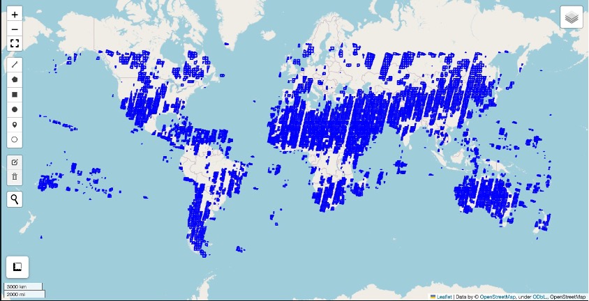
We start by illustrating how SageMaker will be utilized to investigate geospatial knowledge at a world scale. To get began, we comply with the steps outlined in Getting Began with Amazon SageMaker geospatial capabilities. We begin with the specification of the geographical coordinates that outline a bounding field masking the areas of curiosity. This bounding field acts as a filter to pick out solely the related satellite tv for pc photos that cowl the Earth’s land plenty.

import os
import json
import time
import boto3
import geopandas
from shapely.geometry import Polygon
import leafmap.foliumap as leafmap
import sagemaker
import sagemaker_geospatial_map

session = boto3.Session()
execution_role = sagemaker.get_execution_role()
sg_client = session.shopper(service_name="sagemaker-geospatial")
cooridinates =[
    [-179.034845, -55.973798],
    [179.371094, -55.973798],
    [179.371094, 83.780085],
    [-179.034845, 83.780085],
    [-179.034845, -55.973798]
]           
polygon = Polygon(cooridinates)
world_gdf = geopandas.GeoDataFrame(index=[0], crs="epsg:4326", geometry=[polygon])
m = leafmap.Map(heart=[37, -119], zoom=4)
m.add_basemap('Esri.WorldImagery')
m.add_gdf(world_gdf, layer_name="AOI", type={"shade": "purple"})
m

Information acquisition

SageMaker geospatial capabilities present entry to a variety of public geospatial datasets, together with Sentinel-2, Landsat 8, Copernicus DEM, and NAIP. For our vegetation mapping mission, we’ve chosen Sentinel-2 for its world protection and replace frequency. The Sentinel-2 satellite tv for pc captures photos of Earth’s land floor at a decision of 10 meters each 5 days. We choose the primary week of December 2023 on this instance. To ensure we cowl a lot of the seen earth floor, we filter for photos with lower than 10% cloud protection. This fashion, our evaluation is predicated on clear and dependable imagery.

search_rdc_args = {
    "Arn": "arn:aws:sagemaker-geospatial:us-west-2:378778860802:raster-data-collection/public/nmqj48dcu3g7ayw8", # sentinel-2 L2A
    "RasterDataCollectionQuery": {
        "AreaOfInterest": {
            "AreaOfInterestGeometry": {
                "PolygonGeometry": {
                    "Coordinates": [
                        [
                            [-179.034845, -55.973798],
                            [179.371094, -55.973798],
                            [179.371094, 83.780085],
                            [-179.034845, 83.780085],
                            [-179.034845, -55.973798]
                        ]
                    ]
                }
            }
        },
        "TimeRangeFilter": {
            "StartTime": "2023-12-01T00:00:00Z",
            "EndTime": "2023-12-07T23:59:59Z",
        },
        "PropertyFilters": {
            "Properties": [{"Property": {"EoCloudCover": {"LowerBound": 0, "UpperBound": 10}}}],
            "LogicalOperator": "AND",
        },
    }
}

s2_items = []
s2_tile_ids = []
s2_geometries = {
    'id': [],
    'geometry': [],
}
whereas search_rdc_args.get("NextToken", True):
    search_result = sg_client.search_raster_data_collection(**search_rdc_args)
    for merchandise in search_result["Items"]:
        s2_id = merchandise['Id']
        s2_tile_id = s2_id.cut up('_')[1]
        # filtering out tiles cowl the identical space
        if s2_tile_id not in s2_tile_ids:
            s2_tile_ids.append(s2_tile_id)
            s2_geometries['id'].append(s2_id)
            s2_geometries['geometry'].append(Polygon(merchandise['Geometry']['Coordinates'][0]))
            del merchandise['DateTime']
            s2_items.append(merchandise)  

    search_rdc_args["NextToken"] = search_result.get("NextToken")

print(f"{len(s2_items)} distinctive Sentinel-2 photos discovered.")

By using the search_raster_data_collection perform from SageMaker geospatial, we recognized 8,581 distinctive Sentinel-2 photos taken within the first week of December 2023. To validate the accuracy in our choice, we plotted the footprints of those photos on a map, confirming that we had the proper photos for our evaluation.

s2_gdf = geopandas.GeoDataFrame(s2_geometries)
m = leafmap.Map(heart=[37, -119], zoom=4)
m.add_basemap('OpenStreetMap')
m.add_gdf(s2_gdf, layer_name="Sentinel-2 Tiles", type={"shade": "blue"})
m

SageMaker geospatial processing jobs

When querying knowledge with SageMaker geospatial capabilities, we obtained complete particulars about our goal photos, together with the info footprint, properties round spectral bands, and hyperlinks for direct entry. With these hyperlinks, we will bypass conventional reminiscence and storage-intensive strategies of first downloading and subsequently processing photos regionally—a process made much more daunting by the dimensions and scale of our dataset, spanning over 4 TB. Every of the 8,000 photos are massive in measurement, have a number of channels, and are individually sized at roughly 500 MB. Processing a number of terabytes of information on a single machine can be time-prohibitive. Though establishing a processing cluster is an alternate, it introduces its personal set of complexities, from knowledge distribution to infrastructure administration. SageMaker geospatial streamlines this with Amazon SageMaker Processing. We use the purpose-built geospatial container with SageMaker Processing jobs for a simplified, managed expertise to create and run a cluster. With just some strains of code, you may scale out your geospatial workloads with SageMaker Processing jobs. You merely specify a script that defines your workload, the placement of your geospatial knowledge on Amazon Easy Storage Service (Amazon S3), and the geospatial container. SageMaker Processing provisions cluster sources so that you can run city-, country-, or continent-scale geospatial ML workloads.

For our mission, we’re utilizing 25 clusters, with every cluster comprising 20 situations, to scale out our geospatial workload. Subsequent, we divided the 8,581 photos into 25 batches for environment friendly processing. Every batch accommodates roughly 340 photos. These batches are then evenly distributed throughout the machines in a cluster. All batch manifests are uploaded to Amazon S3, prepared for the processing job, so every section is processed swiftly and effectively.

def s2_item_to_relative_metadata_url(merchandise):
    components = merchandise["Assets"]["visual"]["Href"].cut up("/")
    tile_prefix = components[4:-1]
    return "{}/{}.json".format("/".be a part of(tile_prefix), merchandise["Id"])


num_jobs = 25
num_instances_per_job = 20 # most 20

manifest_list = {}
for idx in vary(num_jobs):
    manifest = [{"prefix": "s3://sentinel-cogs/sentinel-s2-l2a-cogs/"}]
    manifest_list[idx] = manifest
# cut up the manifest for N processing jobs
for idx, merchandise in enumerate(s2_items):
    job_idx = idxpercentnum_jobs
    manifest_list[job_idx].append(s2_item_to_relative_metadata_url(merchandise))
    
# add the manifest to S3
sagemaker_session = sagemaker.Session()
s3_bucket_name = sagemaker_session.default_bucket()
s3_prefix = 'processing_job_demo'
s3_client = boto3.shopper("s3")
s3 = boto3.useful resource("s3")

manifest_dir = "manifests"
os.makedirs(manifest_dir, exist_ok=True)

for job_idx, manifest in manifest_list.objects():
    manifest_file = f"{manifest_dir}/manifest{job_idx}.json"
    s3_manifest_key = s3_prefix + "/" + manifest_file
    with open(manifest_file, "w") as f:
        json.dump(manifest, f)

    s3_client.upload_file(manifest_file, s3_bucket_name, s3_manifest_key)
    print("Uploaded {} to {}".format(manifest_file, s3_manifest_key))

With our enter knowledge prepared, we now flip to the core evaluation that may reveal insights into vegetation well being by means of the Normalized Distinction Vegetation Index (NDVI). NDVI is calculated from the distinction between Close to-infrared (NIR) and Pink reflectances, normalized by their sum, yielding values that vary from -1 to 1. Increased NDVI values sign dense, wholesome vegetation, a price of zero signifies no vegetation, and destructive values often level to water our bodies. This index serves as a crucial software for assessing vegetation well being and distribution. The next is an instance of what NDVI appears like.

%%writefile scripts/compute_vi.py

import os
import rioxarray
import json
import gc
import warnings

warnings.filterwarnings("ignore")

if __name__ == "__main__":
    print("Beginning processing")

    input_path = "/choose/ml/processing/enter"
    output_path = "/choose/ml/processing/output"
    input_files = []
    objects = []
    for current_path, sub_dirs, recordsdata in os.stroll(input_path):
        for file in recordsdata:
            if file.endswith(".json"):
                full_file_path = os.path.be a part of(input_path, current_path, file)
                input_files.append(full_file_path)
                with open(full_file_path, "r") as f:
                    objects.append(json.load(f))

    print("Obtained {} enter recordsdata".format(len(input_files)))

    for merchandise in objects:
        print("Computing NDVI for {}".format(merchandise["id"]))
        red_band_url = merchandise["assets"]["red"]["href"]
        nir_band_url = merchandise["assets"]["nir"]["href"]
        scl_mask_url = merchandise["assets"]["scl"]["href"]
        purple = rioxarray.open_rasterio(red_band_url, masked=True)
        nir = rioxarray.open_rasterio(nir_band_url, masked=True)
        scl = rioxarray.open_rasterio(scl_mask_url, masked=True)
        scl_interp = scl.interp(
            x=purple["x"], y=purple["y"]
        )  # interpolate SCL to the identical decision as Pink and NIR bands

        # masks out cloudy pixels utilizing SCL (https://sentinels.copernicus.eu/internet/sentinel/technical-guides/sentinel-2-msi/level-2a/algorithm-overview)
        # class 8: cloud medium chance
        # class 9: cloud excessive chance
        # class 10: skinny cirrus
        red_cloud_masked = purple.the place((scl_interp != 8) & (scl_interp != 9) & (scl_interp != 10))
        nir_cloud_masked = nir.the place((scl_interp != 8) & (scl_interp != 9) & (scl_interp != 10))

        ndvi = (nir_cloud_masked - red_cloud_masked) / (nir_cloud_masked + red_cloud_masked)
        # save the ndvi as geotiff
        s2_tile_id = red_band_url.cut up("/")[-2]
        file_name = f"{s2_tile_id}_ndvi.tif"
        output_file_path = f"{output_path}/{file_name}"
        ndvi.rio.to_raster(output_file_path)
        print("Written output: {}".format(output_file_path))

        # preserve reminiscence utilization low
        del purple
        del nir
        del scl
        del scl_interp
        del red_cloud_masked
        del nir_cloud_masked
        del ndvi

        gc.acquire()

Now we’ve the compute logic outlined, we’re prepared to begin the geospatial SageMaker Processing job. This includes an easy three-step course of: establishing the compute cluster, defining the computation specifics, and organizing the enter and output particulars.

First, to arrange the cluster, we resolve on the quantity and kind of situations required for the job, ensuring they’re well-suited for geospatial knowledge processing. The compute atmosphere itself is ready by deciding on a geospatial picture that comes with all generally used packages for processing geospatial knowledge.

Subsequent, for the enter, we use the beforehand created manifest that lists all picture hyperlinks. We additionally designate an S3 location to avoid wasting our outcomes.

With these components configured, we’re capable of provoke a number of processing jobs without delay, permitting them to function concurrently for effectivity.

from multiprocessing import Course of
import sagemaker
import boto3 
from botocore.config import Config
from sagemaker import get_execution_role
from sagemaker.sklearn.processing import ScriptProcessor
from sagemaker.processing import ProcessingInput, ProcessingOutput

position = get_execution_role()
geospatial_image_uri = '081189585635.dkr.ecr.us-west-2.amazonaws.com/sagemaker-geospatial-v1-0:newest'
# use the retry behaviour of boto3 to keep away from throttling problem
sm_boto = boto3.shopper('sagemaker', config=Config(connect_timeout=5, read_timeout=60, retries={'max_attempts': 20}))
sagemaker_session = sagemaker.Session(sagemaker_client = sm_boto)

def run_job(job_idx):
    s3_manifest = f"s3://{s3_bucket_name}/{s3_prefix}/{manifest_dir}/manifest{job_idx}.json"
    s3_output = f"s3://{s3_bucket_name}/{s3_prefix}/output"
    script_processor = ScriptProcessor(
        command=['python3'],
        image_uri=geospatial_image_uri,
        position=position,
        instance_count=num_instances_per_job,
        instance_type="ml.m5.xlarge",
        base_job_name=f'ca-s2-nvdi-{job_idx}',
        sagemaker_session=sagemaker_session,
    )

    script_processor.run(
        code="scripts/compute_vi.py",
        inputs=[
            ProcessingInput(
                source=s3_manifest,
                destination='/opt/ml/processing/input/',
                s3_data_type="ManifestFile",
                s3_data_distribution_type="ShardedByS3Key"
            ),
        ],
        outputs=[
            ProcessingOutput(
                source="/opt/ml/processing/output/",
                destination=s3_output,
                s3_upload_mode="Continuous"
            )
        ],
    )
    time.sleep(2)

processes = []
for idx in vary(num_jobs):
    p = Course of(goal=run_job, args=(idx,))
    processes.append(p)
    p.begin()
    
for p in processes:
    p.be a part of()

After you launch the job, SageMaker routinely spins up the required situations and configures the cluster to course of the pictures listed in your enter manifest. This whole setup operates seamlessly, with no need your hands-on administration. To observe and handle the processing jobs, you should use the SageMaker console. It provides real-time updates on the standing and completion of your processing duties. In our instance, it took below 20 minutes to course of all 8,581 photos with 500 situations. The scalability of SageMaker permits for quicker processing instances if wanted, just by growing the variety of situations.

Conclusion

The facility and effectivity of SageMaker geospatial capabilities have opened new doorways for environmental monitoring, notably within the realm of vegetation mapping. Via this instance, we showcased methods to course of over 8,500 satellite tv for pc photos in lower than 20 minutes. We not solely demonstrated the technical feasibility, but in addition showcased the effectivity features from utilizing the cloud for environmental evaluation. This method illustrates a big leap from conventional, resource-intensive strategies to a extra agile, scalable, and cost-effective method. The flexibleness to scale processing sources up or down as wanted, mixed with the benefit of accessing and analyzing huge datasets, positions SageMaker as a transformative software within the subject of geospatial evaluation. By simplifying the complexities related to large-scale knowledge processing, SageMaker permits scientists, researchers, and companies stakeholders to focus extra on deriving insights and fewer on infrastructure and knowledge administration.

As we glance to the longer term, the combination of ML and geospatial analytics guarantees to additional improve our understanding of the planet’s ecological techniques. The potential to watch adjustments in actual time, predict future traits, and reply with extra knowledgeable choices can considerably contribute to world conservation efforts. This instance of vegetation mapping is just the start for working planetary-scale ML. See Amazon SageMaker geospatial capabilities to be taught extra.

Concerning the Writer

Xiong Zhou is a Senior Utilized Scientist at AWS. He leads the science crew for Amazon SageMaker geospatial capabilities. His present space of analysis contains LLM analysis and knowledge technology. In his spare time, he enjoys working, enjoying basketball and spending time along with his household.

Anirudh Viswanathan is a Sr Product Supervisor, Technical – Exterior Companies with the SageMaker geospatial ML crew. He holds a Masters in Robotics from Carnegie Mellon College, an MBA from the Wharton College of Enterprise, and is called inventor on over 40 patents. He enjoys long-distance working, visiting artwork galleries and Broadway exhibits.

Janosch Woschitz is a Senior Options Architect at AWS, specializing in AI/ML. With over 15 years of expertise, he helps prospects globally in leveraging AI and ML for progressive options and constructing ML platforms on AWS. His experience spans machine studying, knowledge engineering, and scalable distributed techniques, augmented by a powerful background in software program engineering and business experience in domains corresponding to autonomous driving.

Li Erran Li is the utilized science supervisor at humain-in-the-loop providers, AWS AI, Amazon. His analysis pursuits are 3D deep studying, and imaginative and prescient and language illustration studying. Beforehand he was a senior scientist at Alexa AI, the top of machine studying at Scale AI and the chief scientist at Pony.ai. Earlier than that, he was with the notion crew at Uber ATG and the machine studying platform crew at Uber engaged on machine studying for autonomous driving, machine studying techniques and strategic initiatives of AI. He began his profession at Bell Labs and was adjunct professor at Columbia College. He co-taught tutorials at ICML’17 and ICCV’19, and co-organized a number of workshops at NeurIPS, ICML, CVPR, ICCV on machine studying for autonomous driving, 3D imaginative and prescient and robotics, machine studying techniques and adversarial machine studying. He has a PhD in pc science at Cornell College. He’s an ACM Fellow and IEEE Fellow.

Amit Modi is the product chief for SageMaker MLOps, ML Governance, and Accountable AI at AWS. With over a decade of B2B expertise, he builds scalable merchandise and groups that drive innovation and ship worth to prospects globally.

Kris Efland is a visionary expertise chief with a profitable monitor report in driving product innovation and development for over 20 years. Kris has helped create new merchandise together with shopper electronics and enterprise software program throughout many industries, at each startups and huge corporations. In his present position at Amazon Net Companies (AWS), Kris leads the Geospatial AI/ML class. He works on the forefront of Amazon’s fastest-growing ML service, Amazon SageMaker, which serves over 100,000 prospects worldwide. He just lately led the launch of Amazon SageMaker’s new geospatial capabilities, a strong set of instruments that permit knowledge scientists and machine studying engineers to construct, prepare, and deploy ML fashions utilizing satellite tv for pc imagery, maps, and site knowledge. Earlier than becoming a member of AWS, Kris was the Head of Autonomous Car (AV) Instruments and AV Maps for Lyft, the place he led the corporate’s autonomous mapping efforts and toolchain used to construct and function Lyft’s fleet of autonomous automobiles. He additionally served because the Director of Engineering at HERE Applied sciences and Nokia and has co-founded a number of startups..