With the looks of ChatGPT, the world acknowledged the highly effective potential of huge language fashions, which may perceive pure language and reply to consumer requests with excessive accuracy. Within the abbreviation of Llm, the primary letter L stands for Giant, reflecting the huge variety of parameters these fashions sometimes have.
Trendy LLMs typically include over a billion parameters. Now, think about a state of affairs the place we need to adapt an LLM to a downstream process. A typical strategy consists of fine-tuning, which includes adjusting the mannequin’s current weights on a brand new dataset. Nonetheless, this course of is extraordinarily gradual and resource-intensive — particularly when run on a neighborhood machine with restricted {hardware}.

Throughout fine-tuning, some neural community layers may be frozen to cut back coaching complexity, this strategy nonetheless falls brief at scale as a consequence of excessive computational prices.
To handle this problem, on this article we’ll discover the core rules of Lora (Low-Rank Adaptation), a well-liked approach for decreasing the computational load throughout fine-tuning of huge fashions. As a bonus, we’ll additionally check out QLoRA, which builds on LoRA by incorporating quantization to additional improve effectivity.
Neural community illustration
Allow us to take a totally linked neural community. Every of its layers consists of n neurons absolutely linked to m neurons from the next layer. In whole, there are n ⋅ m connections that may be represented as a matrix with the respective dimensions.

When a brand new enter is handed to a layer, all we’ve got to do is to carry out matrix multiplication between the burden matrix and the enter vector. In follow, this operation is extremely optimized utilizing superior linear algebra libraries and infrequently carried out on whole batches of inputs concurrently to hurry up computation.
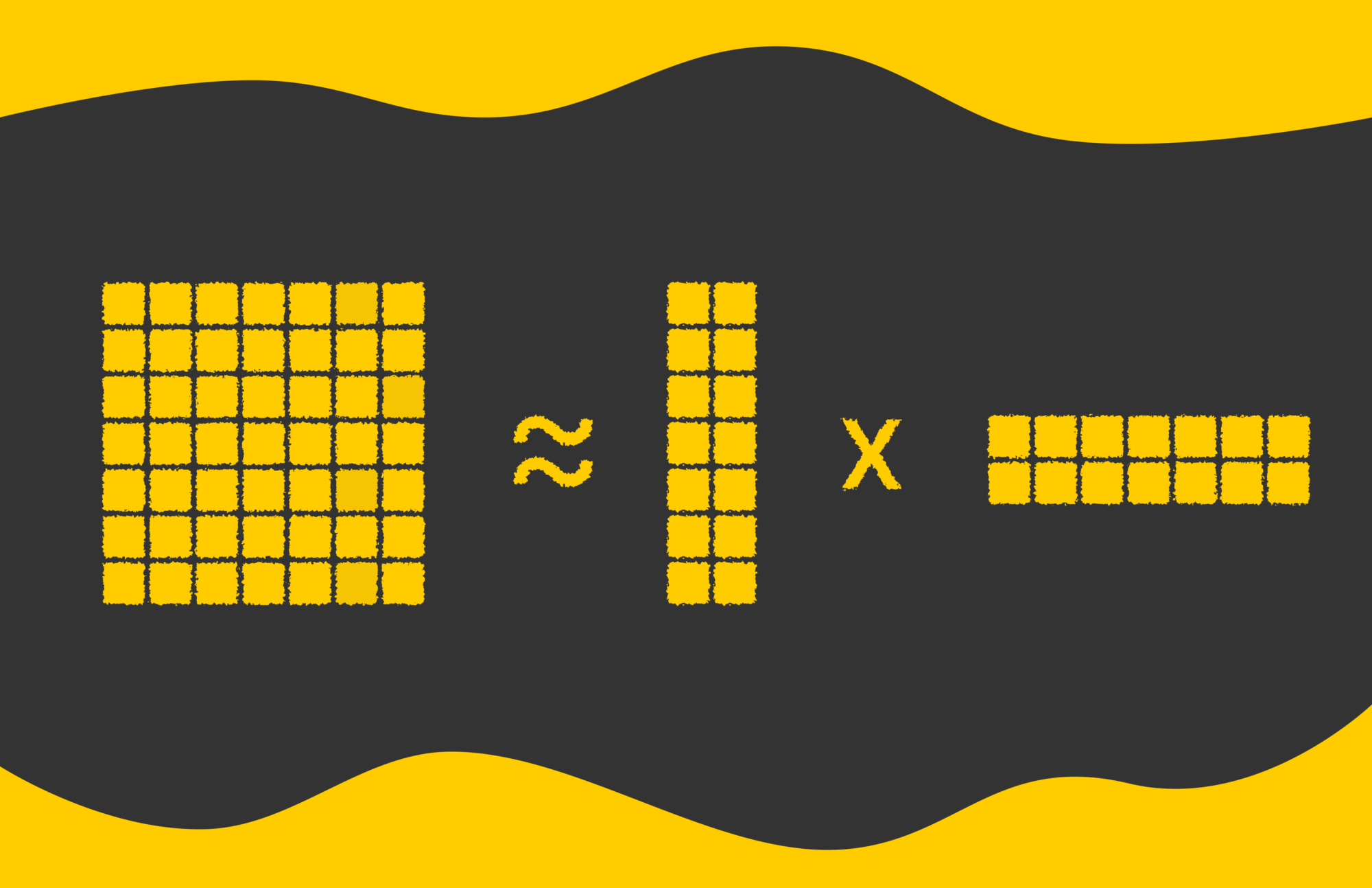
Multiplication trick
The burden matrix in a neural community can have extraordinarily giant dimensions. As an alternative of storing and updating the total matrix, we will factorize it into the product of two smaller matrices. Particularly, if a weight matrix has dimensions n × m, we will approximate it utilizing two matrices of sizes n × okay and okay × m, the place okay is a a lot smaller intrinsic dimension (okay << n, m).
As an illustration, suppose the unique weight matrix is 8192 × 8192, which corresponds to roughly 67M parameters. If we select okay = 8, the factorized model will encompass two matrices: one among measurement 8192 × 8 and the opposite 8 × 8192. Collectively, they include solely about 131K parameters — greater than 500 occasions fewer than the unique, drastically decreasing reminiscence and compute necessities.

The apparent draw back of utilizing smaller matrices to approximate a bigger one is the potential loss in precision. After we multiply the smaller matrices to reconstruct the unique, the ensuing values won’t precisely match the unique matrix parts. This trade-off is the worth we pay for considerably decreasing reminiscence and computational calls for.
Nonetheless, even with a small worth like okay = 8, it’s typically potential to approximate the unique matrix with minimal loss in accuracy. In truth, in follow, even values as little as okay = 2 or okay = 4 may be generally used successfully.
LoRA
The thought described within the earlier part completely illustrates the core idea of LoRA. LoRA stands for Low-Rank Adaptation, the place the time period low-rank refers back to the strategy of approximating a big weight matrix by factorizing it into the product of two smaller matrices with a a lot decrease rank okay. This strategy considerably reduces the variety of trainable parameters whereas preserving many of the mannequin’s energy.
Coaching
Allow us to assume we’ve got an enter vector x handed to a totally linked layer in a neural community, which earlier than fine-tuning, is represented by a weight matrix W. To compute the output vector y, we merely multiply the matrix by the enter: y = Wx.
Throughout fine-tuning, the aim is to regulate the mannequin for a downstream process by modifying the weights. This may be expressed as studying a further matrix ΔW, such that: y = (W + ΔW)x = Wx + ΔWx. As we noticed the multiplication trick above, we will now exchange ΔW by multiplication BA, so we finally get: y = Wx + BAx. Consequently, we freeze the matrix Wand remedy the Optimization process to seek out matrices A and B that absolutely include a lot much less parameters than ΔW!
Nonetheless, direct calculation of multiplication (BA)x throughout every ahead move may be very gradual because of the the truth that matrix multiplication BA is a heavy operation. To keep away from this, we will leverage associative property of matrix multiplication and rewrite the operation as B(Ax). The multiplication of A by x leads to a vector that might be then multiplied by B which additionally finally produces a vector. This sequence of operations is far sooner.

By way of backpropagation, LoRA additionally gives a number of advantages. Although a gradient for a single neuron nonetheless takes almost the identical quantity of operations, we now take care of a lot fewer parameters in our community, which suggests:
- we have to compute far fewer gradients for A and B than would initially have been required for W.
- we now not have to retailer a large matrix of gradients for W.
Lastly, to compute y, we simply want so as to add the already calculated Wx and BAx. There are not any difficulties right here since matrix addition may be simply parallelized.
As a technical element, earlier than fine-tuning, matrix A is initialized utilizing a Gaussian distribution, and matrix B is initialized with zeros. Utilizing a zero matrix for B originally ensures that the mannequin behaves precisely as earlier than, as a result of BAx = 0 · Ax = 0, so y stays equal to Wx.
This makes the preliminary part of fine-tuning extra secure. Then, throughout backpropagation, the mannequin regularly adapts its weights for A and B to study new data.
After coaching
After coaching, we’ve got calculated the optimum matrices A and B. All we’ve got to do is multiply them to compute ΔW, which we then add to the pretrained matrix W to acquire the ultimate weights.
Whereas the matrix multiplication BA may appear to be a heavy operation, we solely carry out it as soon as, so it mustn’t concern us an excessive amount of! Furthermore, after the addition, we now not have to retailer A, B, or ΔW.
Subtlety
Whereas the concept of LoRA appears inspiring, a query may come up: throughout regular coaching of neural networks, why can’t we straight symbolize y as BAx as a substitute of utilizing a heavy matrix W to calculate y = Wx?
The issue with simply utilizing BAx is that the mannequin’s capability can be a lot decrease and certain inadequate for the mannequin to study successfully. Throughout coaching, a mannequin must study huge quantities of data, so it naturally requires numerous parameters.
In LoRA optimization, we deal with Wx because the prior data of the big mannequin and interpret ΔWx = BAx as task-specific data launched throughout fine-tuning. So, we nonetheless can not deny the significance of W within the mannequin’s general efficiency.
Adapter
Finding out LLM concept, you will need to point out the time period “adapter” that seems in lots of LLM papers.
Within the LoRA context, an adapter is a mix of matrices A and B which can be used to unravel a specific downstream process for a given matrix W.
For instance, allow us to suppose that we’ve got skilled a matrix W such that the mannequin is ready to perceive pure language. We are able to then carry out a number of impartial LoRA optimizations to tune the mannequin on completely different duties. Consequently, we acquire a number of pairs of matrices:
- (A₁, B₁) — adapter used to carry out question-answering duties.
- (A₂, B₂) — adapter used for textual content summarization issues.
- (A₃, B₃) — adapter skilled for chatbot growth.

Provided that, we will retailer a single matrix and have as many adapters as we would like for various duties! Since matrices A and B are tiny, they’re very straightforward to retailer.
Adapter ajustement in actual time
The beauty of adapters is that we will change them dynamically. Think about a situation the place we have to develop a chatbot system that permits customers to decide on how the bot ought to reply primarily based on a particular character, resembling Harry Potter, an offended hen, or Cristiano Ronaldo.
Nonetheless, system constraints could forestall us from storing or fine-tuning three separate giant fashions as a consequence of their giant measurement. What’s the answer?
That is the place adapters come to the rescue! All we want is a single giant mannequin W and three separate adapters, one for every character.

We preserve in reminiscence solely matrix W and three matrix pairs: (A₁, B₁), (A₂, B₂), (A₃, B₃). At any time when a consumer chooses a brand new character for the bot, we simply need to dynamically exchange the adapter matrix by performing matrix addition between Wand (Aᵢ, Bᵢ). Consequently, we get a system that scales extraordinarily nicely if we have to add new characters sooner or later!
QLoRA
QLoRA is one other widespread time period whose distinction from LoRA is barely in its first letter, Q, which stands for “quantized”. The time period “quantization” refers back to the decreased variety of bits which can be used to retailer weights of neurons.
As an illustration, we will symbolize neural community weights as floats requiring 32 bits for every particular person weight. The thought of quantization consists of compressing neural community weights to a smaller precision with out vital loss or influence on the mannequin’s efficiency. So, as a substitute of utilizing 32 bits, we will drop a number of bits to make use of, for example, solely 16 bits.

Talking of QLoRA, quantization is used for the pretrained matrix W to cut back its weight measurement.
*Bonus: prefix-tuning
Prefix-tuning is an attention-grabbing various to LoRA. The thought additionally consists of utilizing adapters for various downstream duties however this time adapters are built-in inside the eye layer of the Transformer.
Extra particularly, throughout coaching, all mannequin layers develop into frozen aside from these which can be added as prefixes to a number of the embeddings calculated inside consideration layers. Compared to LoRA, prefix tuning doesn’t change mannequin illustration, and on the whole, it has a lot fewer trainable parameters. As beforehand, to account for the prefix adapter, we have to carry out addition, however this time with fewer parts.
Until given very restricted computational and reminiscence constraints, LoRA adapters are nonetheless most well-liked in lots of instances, in comparison with prefix tuning.
Conclusion
On this article, we’ve got checked out superior LLM ideas to know how giant fashions may be effectively tuned with out computational overhead. LoRA’s class in compressing the burden matrix via matrix decomposition not solely permits fashions to coach sooner but in addition requires much less reminiscence area. Furthermore, LoRA serves as a wonderful instance to exhibit the concept of adapters that may be flexibly used and switched for downstream duties.
On high of that, we will add a quantization course of to additional scale back reminiscence area by lowering the variety of bits required to symbolize every neuron.
Lastly, we explored one other various known as “prefix tuning”, which performs the identical function as adapters however with out altering the mannequin illustration.
Sources
All photos are by the creator except famous in any other case.


