
, I mentioned the best way to create your first DataFrame utilizing Pandas. I discussed that the very first thing you might want to grasp is Knowledge constructions and arrays earlier than transferring on to information evaluation with Python.
Pandas is a superb library for information manipulation and retrieval. Mix it with Numpy and Seaborne, and also you’ve bought your self a powerhouse for information evaluation.
On this article, I’ll be strolling you thru sensible methods to filter information in pandas, beginning with easy circumstances and transferring on to highly effective strategies like .isin(), .str.startswith(), and .question(). By the top, you’ll have a toolkit of filtering methods you’ll be able to apply to any dataset.
With out additional ado, let’s get into it!
Importing our information
Okay, to start out, I’ll import our pandas library
# importing the pandas library
import pandas as pd
That’s the one library I’ll want for this use case
Subsequent, I’ll import the dataset. The dataset comes from ChatGPT, btw. It consists of fundamental gross sales transaction data. Let’s check out our dataset.
# testing our information
df_sales = pd.read_csv('sales_data.csv')
df_sales
Right here’s a preview of the information

It consists of fundamental gross sales data with columns OrderId, Buyer, Product, Class, Amount, Value, OrderDate and Area.
Alright, let’s start our filtering!
Filtering by a single situation
Let’s attempt to choose all data from a specific class. As an illustration, I need to know what number of distinctive orders had been made within the Electronics class. To try this, it’s fairly easy
# Filter by a single situation
# Instance: All orders from the “Electronics” class.
df_sales[‘Category’] == ‘Electronics’
In Python, you might want to distinguish between the = operator and the == operator.
= is used to assign a price to a variable.
As an illustration
x = 10 # Assigns the worth 10 to the variable x== alternatively is used to match two values collectively. As an illustration
a = 3
b = 3
print(a == b) # Output: True

c = 5
d = 10
print(c == d) # Output: False
With that mentioned, let’s apply the identical notion to the filtering I did above
# Filter by a single situation
# Instance: All orders from the “Electronics” class.
df_sales[‘Category’] == ‘Electronics’
Right here, I’m mainly telling Python to look by means of our whole report to discover a class named Electronics. When it finds a match, it shows a Boolean outcome, True or False. Right here’s the outcome

As you’ll be able to see. We’re getting a Boolean output. True means Electronics exists, whereas False means the latter. That is okay and all, however it may possibly turn into complicated when you’re coping with numerous data. Let’s repair that.
# Filter by a single situation
# Instance: All orders from the “Electronics” class.
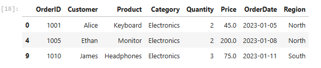
df_sales[df_sales[‘Category’] == ‘Electronics’]Right here, I simply wrapped the situation within the DataFrame. And with that, we get this output

A lot better, proper? Let’s transfer on
Filter rows by numeric situation
Let’s attempt to retrieve data the place the order amount is bigger than 2. It’s fairly easy.
# Filter rows by numeric situation
# Instance: Orders the place Amount > 2
df_sales[‘Quantity’] > 2
Right here, I’m utilizing the better than > operator. Just like our output above, we’re gonna get a Boolean outcome with True and False values. Let’s repair it up actual fast.

And there we go!
Filter by date situation
Filtering by date is simple. As an illustration.
# Filter by date situation
# Instance: Orders positioned after “2023–01–08”
df_sales[df_sales[“OrderDate”] > “2023–01–08”]
This checks for orders positioned after January 8, 2023. And right here’s the output.

The cool factor about Pandas is that it converts string information varieties to dates routinely. In circumstances the place you encounter an error. You would possibly need to convert to a date earlier than filtering utilizing the to_datetime() perform. Right here’s an instance
df[“OrderDate”] = pd.to_datetime(df[“OrderDate”])This converts our OrderDate column to a date information kind. Let’s kick issues up a notch.
Filtering by A number of Circumstances (AND, OR, NOT)
Pandas permits us to filter on a number of circumstances utilizing logical operators. Nonetheless, these operators are completely different from Python’s built-in operators like (and, or, not). Listed below are the logical operators you’ll be working with probably the most
& (Logical AND)
The ampersand (&) image represents AND in pandas. We use this after we’re making an attempt to fulfil two circumstances. On this case, each circumstances need to be true. As an illustration, let’s retrieve orders from the “Furnishings” class the place Value > 500.
# A number of circumstances (AND)
# Instance: Orders from “Furnishings” the place Value > 500
df_sales[(df_sales[“Category”] == “Furnishings”) & (df_sales[“Price”] > 500)]
Let’s break this down. Right here, now we have two circumstances. One which retrieves orders within the Furnishings class and one other that filters for costs > 500. Utilizing the &, we’re capable of mix each circumstances.
Right here’s the outcome.

One report was managed to be retrieved. it, it meets our situation. Let’s do the identical for OR
| (Logical OR)
The |,vertical bar image is used to characterize OR in pandas. On this case, a minimum of one of many corresponding parts ought to be True. As an illustration, let’s retrieve data with orders from the “North” area OR “East” area.
# A number of circumstances (OR)
# Instance: Orders from “North” area OR “East” area.
df_sales[(df_sales[“Region”] == “North”) | (df_sales[“Region”] == “East”)]
Right here’s the output

Filter with isin()
Let’s say I need to retrieve orders from a number of prospects. I may all the time use the & operator. As an illustration
df_sales[(df_sales[‘Customer’] == ‘Alice’) | (df_sales[‘Customer’] == ‘Charlie’)]Output:

Nothing mistaken with that. However there’s a greater and simpler means to do that. That’s through the use of the isin() perform. Right here’s the way it works
# Orders from prospects ["Alice", "Diana", "James"].
df_sales[df_sales[“Customer”].isin([“Alice”, “Diana”, “James”])]
Output:

The code is far simpler and cleaner. Utilizing the isin() perform, I can add as many parameters as I need. Let’s transfer on to some extra superior filtering.
Filter utilizing string matching
One among Pandas’ highly effective however underused features is string matching. It helps a ton in information cleansing duties whenever you’re making an attempt to look by means of patterns within the data in your DataFrame. Just like the LIKE operator in SQL. As an illustration, let’s retrieve prospects whose title begins with “A”.
# Prospects whose title begins with "A".
df_sales[df_sales[“Customer”].str.startswith(“A”)]
Output:

Pandas offers you the .str accessor to make use of string features. Right here’s one other instance
# Merchandise ending with “prime” (e.g., Laptop computer).
df_sales[df_sales[“Product”].str.endswith(“prime”)]
Output:

Filter utilizing question() methodology
When you’re coming from a SQL background, this methodology can be so useful for you. Let’s attempt to retrieve orders from the electronics class the place the amount > 2. It could actually all the time go like this.
df_sales[(df_sales[“Category”] == “Electronics”) & (df_sales[“Quantity”] >= 2)]Output:
However when you’re somebody making an attempt to usher in your SQL sauce. It will give you the results you want as an alternative
df.question(“Class == ‘Electronics’ and Amount >= 2”)You’ll get the identical output above. Fairly much like SQL when you ask me, and also you’ll be capable of ditch the & image. I’m gonna be utilizing this methodology very often.
Filter by column values in a spread
Pandas permits you to retrieve a spread of values. As an illustration, Orders the place the Value is between 50 and 500 would go like this
# Orders the place the Value is between 50 and 500
df_sales[df_sales[“Price”].between(50, 500)]
Output:

Fairly easy.
Filter lacking values (NaN)
That is most likely probably the most useful perform as a result of, as an information analyst, one of many information cleansing duties you’ll be engaged on probably the most is filtering out lacking values. To do that in Pandas is simple. That’s through the use of the notna() perform. Let’s filter rows the place Value is just not null.
# filter rows the place Value is just not null.
df_sales[df_sales[“Price”].notna()]
Output:

And there you go. I don’t actually discover the distinction, although, however I’m gonna belief it’s completed.
Conclusion
The subsequent time you open a messy CSV and surprise “The place do I even begin?”, strive filtering first. It’s the quickest solution to minimize by means of the noise and discover the story hidden in your information.
The transition to Python for information evaluation used to really feel like an enormous step, coming from a SQL background. However for some purpose, Pandas appears means simpler and fewer time-consuming for me for filtering information
The cool half about that is that these similar methods work regardless of the dataset — gross sales numbers, survey responses, internet analytics, you title it.
I hope you discovered this text useful.
I write these articles as a solution to check and strengthen my very own understanding of technical ideas — and to share what I’m studying with others who is perhaps on the identical path. Be at liberty to share with others. Let’s study and develop collectively. Cheers!
Be at liberty to say hello on any of those platforms


