

Most giant language fashions (LLMs) use transformer architectures with softmax consideration. Throughout inference, their key-value (KV) cache grows with the dialog or doc context. This may scale back concurrency, improve serving price, and drive agentic functions to discard helpful historical past.
i14 designed Laplace 3B as a linear consideration different. Its recurrent state stays at 29.5 MB per sequence, impartial of context size. Working with AWS, i14 used native PyTorch help by means of TorchNeuron Native to deliver this practice structure to AWS Trainium2. This preserved its Gated Linear Consideration (GLA) design and Muon optimizer.
On one trn2.48xlarge occasion, Laplace 3B skilled at about 120,000 tokens per second. The mannequin served 11,544 output tokens per second throughout 1,280 concurrent sequences. This publish explains the mannequin design, the adjustments i14 made for Trainium2, and the coaching and inference outcomes.
About i14
i14 is an AI analysis and expertise firm that develops mannequin architectures, elements, and runtimes. Its work attracts on AI, computational cognitive science, and analysis into how organic methods be taught over time. i14 applies these concepts to fashions that may retain long-range context with out permitting serving state to develop with each token.
Why linear consideration fashions?
Transformer softmax consideration compares tokens throughout the context. Throughout coaching, this computation grows quadratically with sequence size. Throughout inference, the KV cache grows because the mannequin processes extra tokens.
Linear consideration reorganizes the computation round a recurrent state that’s up to date for every token. Laplace 3B makes use of GLA to compress prior context right into a fixed-size matrix state. This adjustments coaching consideration from O(T2) to O(T) and retains inference state fastened at 29.5 MB per sequence.
| Consideration | Transformer softmax consideration | Laplace 3B with GLA |
| Coaching consideration | Builds pairwise token scores with O(T2) scaling | Updates chunked recurrent state with O(T) scaling |
| Inference reminiscence | KV cache grows with context | Recurrent state stays fastened in dimension |
| Longer contexts | Every sequence consumes extra accelerator reminiscence | Context size doesn’t improve recurrent-state allocation |
| Implementation | Makes use of broadly optimized consideration kernels | Requires architecture-specific kernels and compiler tuning |
Linear consideration compresses historical past quite than retaining each key and worth. You need to due to this fact consider retrieval high quality in your workloads. The fastened state can profit long-running brokers, large-document evaluation, and functions that want persistent reminiscence with predictable serving necessities.
How i14 tailored Laplace 3B for AWS Trainium2
The unique implementation of Laplace 3B used GPU-optimized Triton kernels. The AWS Generative AI Innovation Heart (GenAIIC) staff first rewrote the GLA kernel with customary PyTorch operators for Trainium2. After evaluating each approaches, the staff selected the beta model of TorchNeuron Native, the native PyTorch backend for AWS Trainium, as a result of it carried out higher.
The implementation required three adjustments:
- Utilizing native PyTorch for the GLA consideration kernel. The staff changed the GPU-specific fused_chunk_simple_gla Triton kernel with customary PyTorch operators, utilizing 16 chunks of 128 tokens to match the 128 partitions of the NeuronCore on-chip buffer.
- Redesigning how Muon communicates. Two all_to_all collectives in MuonFSDP2 reduce per-rank visitors by 24 instances and raised throughput by 1.63 instances.
- Compiling the sequential backward cross. The staff statically unrolled the 16 chunk steps of the GLA recurrence to suit the graph-size and on-chip reminiscence limits of the compiler.
The engineering challenges part describes every change intimately.
Why AWS Trainium accelerators?
AWS Trainium is a household of AWS machine studying (ML) accelerators designed for mannequin coaching and inference. A trn2.48xlarge occasion combines 16 Trainium2 chips, 64 logical NeuronCores, high-bandwidth reminiscence, and NeuronLink-v3 connectivity. These assets help the distributed coaching and inference configurations described on this publish.
Three properties of Trainium2 formed the implementation: software-managed on-chip reminiscence (Problem 1), a quick chip-to-chip interconnect (Problem 2), and a static compiler (Problem 3). The compiler traces the GLA recurrence as a hard and fast graph.
Software program-managed on-chip reminiscence. Every NeuronCore has a 28 MiB State Buffer (SBUF) with 128 partitions and a 2 MiB partial-sum buffer (PSUM). The PSUM is wired to a 128×128 systolic Tensor Engine, alongside separate vector and scalar items. The SBUF will not be a cache: the compiler schedules each HBM-to-SBUF switch forward of time, so the information is in place with no evictions or misses (Determine 1).
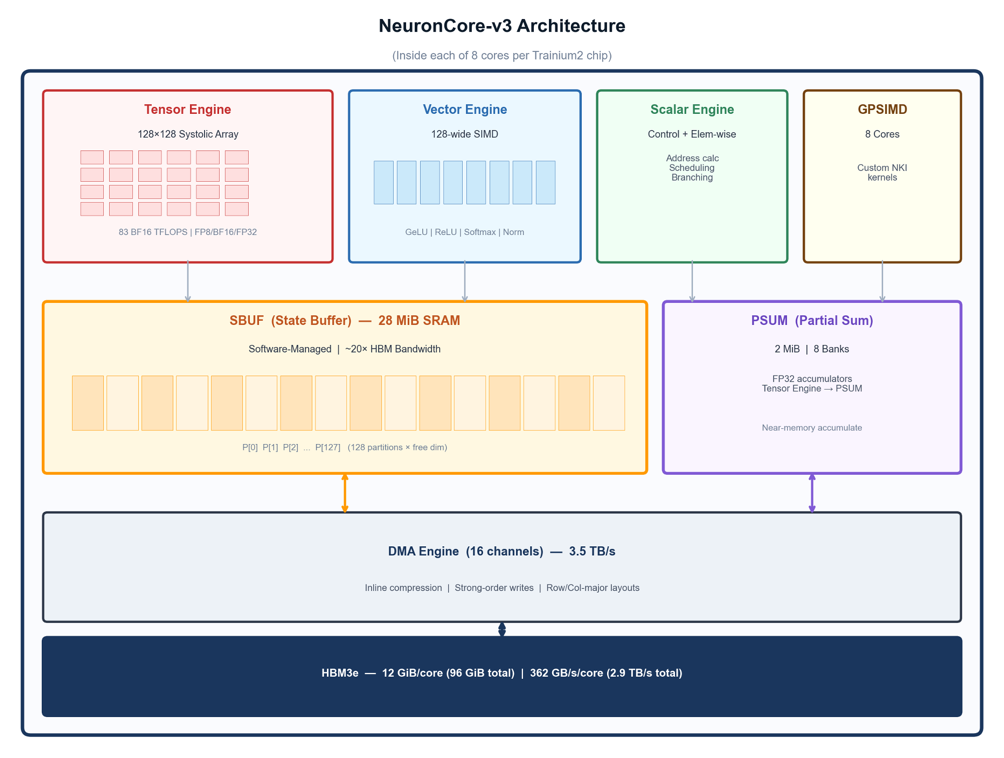
Determine 1: NeuronCore-v3 inner structure. Software program-managed SBUF (28 MiB, 128 partitions), Tensor Engine (128×128 systolic array), Vector Engine, Scalar Engine, and GPSIMD cores.
i14 and the Laplace 3B structure
Laplace 3B is the 24-layer i14 decoder, the place each layer replaces softmax consideration with Easy GLA. Determine 2 follows one layer from the enter xt on the prime to the output xt + 1 on the backside. This part explains every module: normalization and convolution, the QKVG projection, the GLA mixer, and the feed-forward channel mixer.
Normalization and convolution. Every token’s residual-stream vector xt ∈ ℝD (D = 3, 072) passes by means of a LayerNorm and a depth-wise causal Conv1d of width ok = 4 with SiLU. This provides each place a 4-gram abstract earlier than the mixer. The GLA mixer then does content-based retrieval over the entire historical past by means of its decaying state.
QKVG projection. The post-conv output goes by means of one fused matrix Wqokvg ∈ ℝ9, 216 × 3, 072, the place 9, 216 = H × (2dok + 2dv). It splits into 4 per-token streams: queries qt, keys okt, values vt, and a gate gt (H = 16, dok = 96, dv = 192). The gate is used after the mixer.
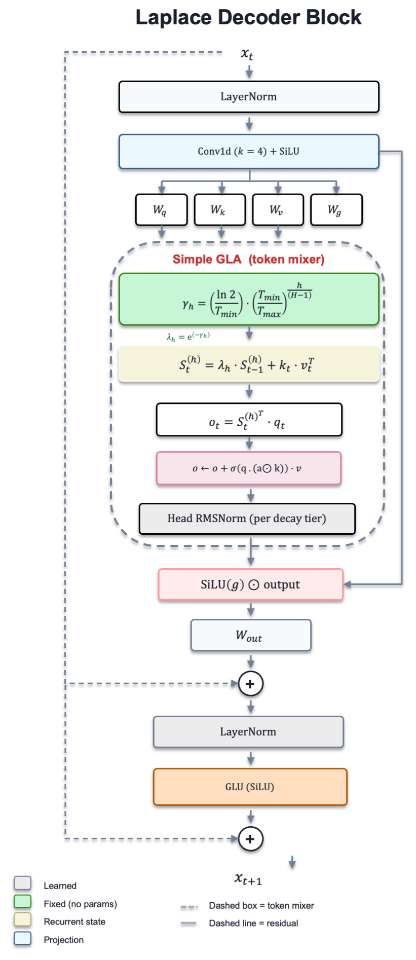
Determine 2: Laplace decoder layer structure. Inexperienced = fastened (no params), grey = realized, yellow = recurrent state, blue = projection.
GLA mixer. Every head h retains a matrix state St(h) of dimension dok × dv (96 × 192), a compressed, decaying file of previous key-value pairs. At every token, it updates as:
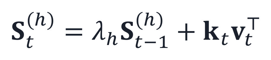
GLA recurrent-state replace equation
Right here λh is the fastened per-head decay, and oktvt⊤ is the rank-1 outer product that writes the present key-value pair into the state. The readout queries the state:
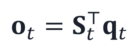
GLA state-readout equation
Subsequent, a self-augmentation step provides a gated copy of the worth to every head’s output:

GLA self-augmentation equation
Right here σ is the sigmoid and ⊙ is the element-wise product. The gate is the question dotted with a realized per-channel rescaling of the important thing, the place a is the realized scale (aug_balance). At initialization, a = 0, which provides a half-strength skip of the worth. The per-head outputs cross by means of a Head RMSNorm inside every decay tier, are concatenated, gated by SiLU(gt), and projected by Wout ∈ ℝD × D again to the residual stream.
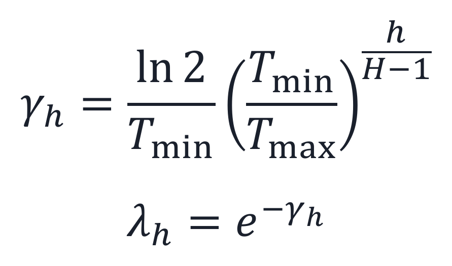
Decay schedule. The per-head decay price λh controls how briskly a head forgets previous tokens. It’s fastened at initialization (not realized) and set by a geometrical schedule. The schedule offers the 16 heads a ramification of reminiscence lengths and defines every head’s log-decay price γh:
GLA decay schedule equations
Decay schedule’s attain. For this mannequin, Tmin = 1 and Tmax = 2, 048. Head 0 due to this fact has λ0 = 0.5 (half-life of 1 token), and head 15 has λ15 ≈ 0.9997 (half-life of two,048 tokens). Heads are grouped into tiers, every sharing a Head RMSNorm.
Channel mixer (FFN). After the eye block and its residual, a second LayerNorm feeds a GLU (SiLU) FFN with interior dimension 8,192. Its three matrices are two up-projections W1, W2 ∈ ℝ8, 192 × D and one down-projection W3 ∈ ℝD × 8, 192. A second residual follows.
The state S(h) is fastened at dok × dv = 96 × 192 per head no matter sequence size. In consequence, inference is O(1) per token, and coaching is O(T) quite than O(T2).
| Parameter | Worth |
| Parameters | 3.028B whole (2.718B Muon + 309.6M AdamW) |
| Layers | 24 decoder layers, D = 3, 072 hidden dim |
| Heads | 16 heads, dok = 96 (half-width Q/Okay), dv = 192 (full-width V) |
| Mixer | Easy GLA with fastened geometric decay (Tmin = 1, Tmax = 2, 048) |
| Conv | Depth-wise causal Conv1d, kernel width 4, SiLU |
| FFN | GLU (SiLU), interior dim 8,192 |
| Norm | LayerNorm pre-attn + Head RMSNorm (per tier) + LayerNorm pre-FFN |
| Vocab | 50,304 (padded to a number of of 64) |
| Sequence | 2,048 |
| Coaching knowledge | 100B tokens, FineWeb-Edu |
| Optimizer | Muon for 2D weight matrices; AdamW for embeddings, norms |
| Batch dimension | 524,288 tokens/step, cosine LR, 3,815-step warmup |
Engineering challenges
Every of the three adjustments raised its personal engineering problem.
Problem 1: Utilizing native PyTorch on Trainium for GLA
On GPU, GLA runs because the fused Triton kernel fused_chunk_simple_gla from the flash-linear-attention library. The GenAIIC staff re-expressed it with customary PyTorch operators working by means of TorchNeuron Native, as specific loops over fixed-size chunks. The chunk rely is fastened at compile time and units the backward-unroll depth. The staff makes use of fla_num_chunks = 16, so every chunk holds C = 128 tokens.
Inside every chunk c, the intra-chunk output is masked linear consideration, and the working state S provides earlier context:

Chunked GLA intra-chunk output
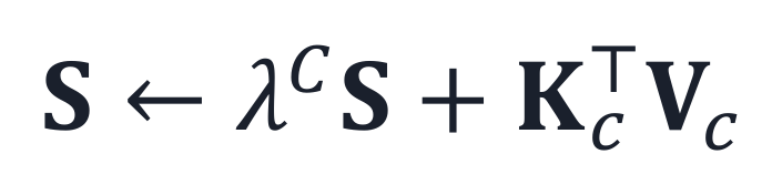
The state then advances to the following chunk:
Chunked GLA state replace
Right here λC is the per-head decay compounded over the chunk. The 16 intra-chunk computations run in parallel, and solely the state replace is sequential (Determine 3).
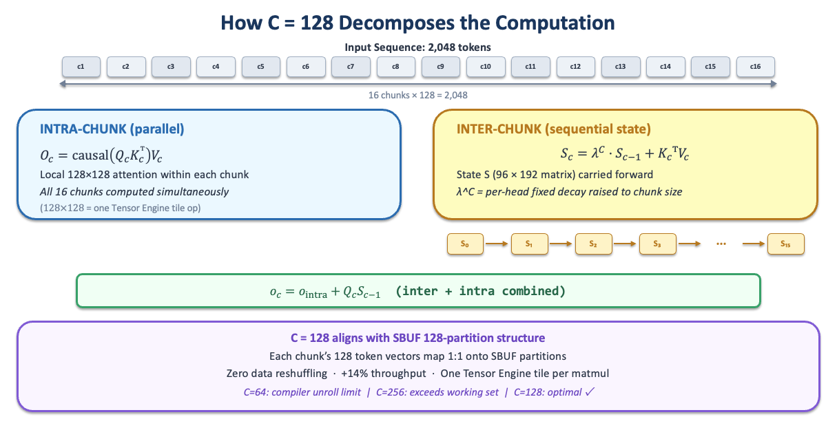
Determine 3: GLA chunked recurrence with parallel intra-chunk consideration and a sequential state chain.
As a result of the SBUF has 128 partitions, every 128-token chunk maps one token per partition, with no padding or cross-partition motion. This alignment elevated measured throughput by 14 p.c (Determine 4).
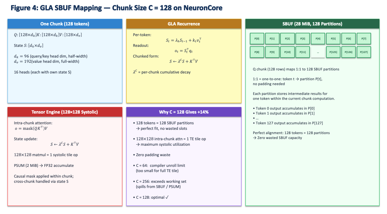
Determine 4: Chunk dimension C = 128 maps one-to-one onto the 128 SBUF partitions.
Problem 2: Distributed Muon orthogonalization underneath FSDP2
Muon orthogonalizes every gradient earlier than the replace. For every of the 96 two-dimensional weight matrices (2.718 billion parameters), it runs 5 Newton–Schulz iterations (Algorithm 1).
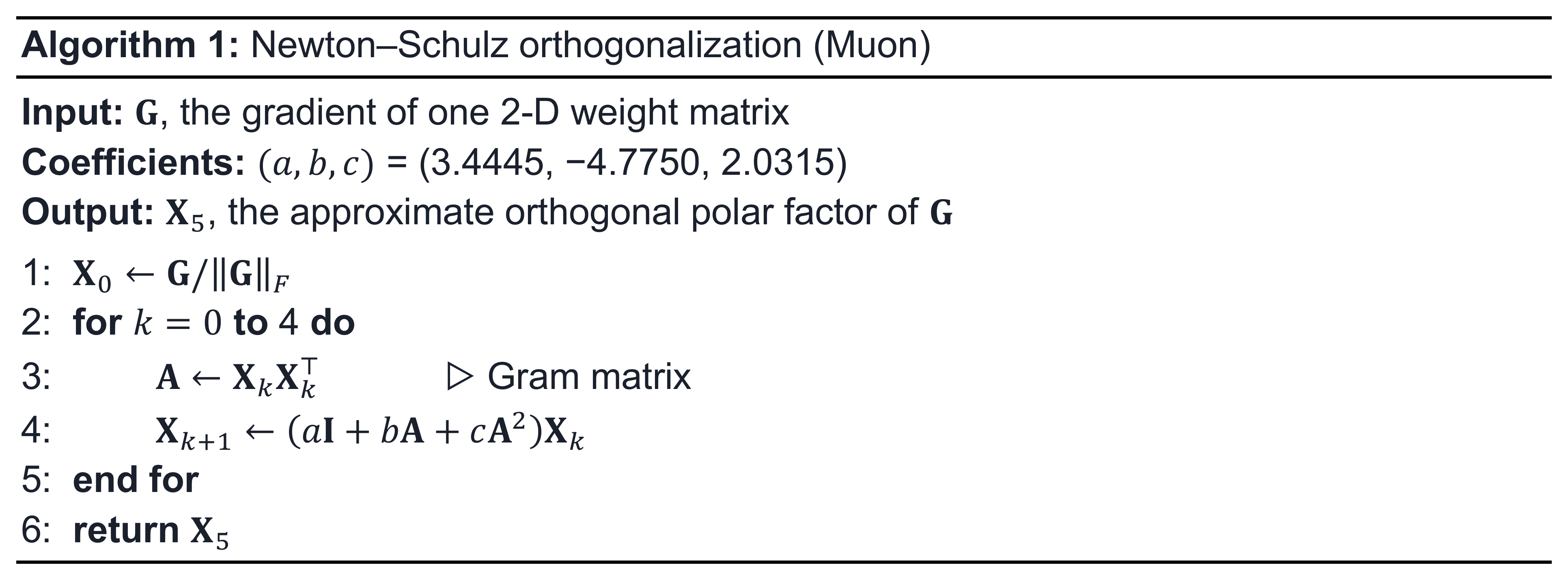
The Newton-Schulz algorithm
The distributed downside. The Gram matrix A = XX⊤ correlates each row of the burden with each different row. Underneath Totally Sharded Knowledge Parallel (FSDP2), every of the 64 ranks holds only one/64 of the rows. A shard-local XX⊤ due to this fact yields solely a diagonal block and drops each cross-shard time period (Determine 5).
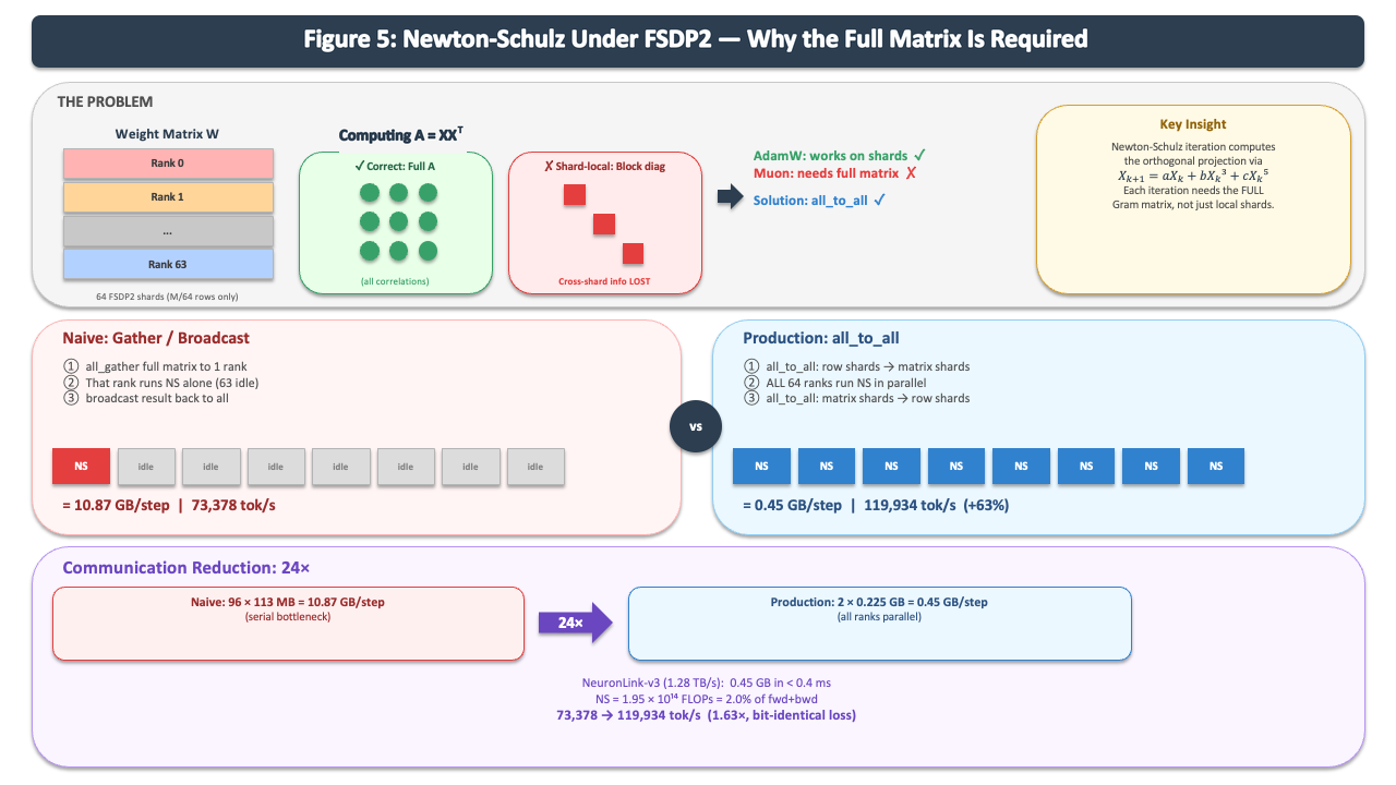
Determine 5: Newton–Schulz underneath FSDP2: the shard-local Gram block, and collect/broadcast in contrast with all_to_all.
Naive strategy: Collect and broadcast. Each rank gathers the total gradient (5.44 GB), one rank runs Newton–Schulz, and it broadcasts the outcome. This strikes 10.87 GB per step whereas the opposite 63 ranks wait.
Manufacturing strategy: all_to_all transposition. In MuonFSDP2, one all_to_all offers every rank just a few full matrices, all 64 ranks run Newton–Schulz in parallel, and a second all_to_all returns the outcomes. Per-rank visitors drops to 0.45 GB, 24 instances much less. Throughput rises from 73,378 to 119,934 tokens per second, 1.63 instances increased, with a bit-identical loss curve (Determine 6).
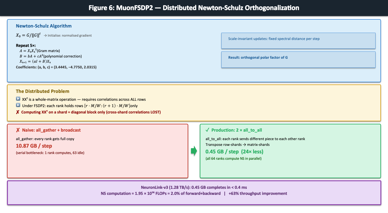
Determine 6: Per-step communication quantity: 10.87 GB with all_gather in contrast with 0.45 GB with all_to_all.
Communication price. Newton–Schulz is simply about 2 p.c of the FLOPs in a coaching step (1.95 × 10¹⁴ of 9.53 × 10¹⁵), so communication was the bottleneck. Over NeuronLink-v3 at 1.28 TB/s, the 0.45 GB alternate takes underneath 0.4 ms of the roughly 4.4-second step.
Problem 3: Backward-pass unrolling for a sequential recurrence
The backward cross differentiates by means of all 16 sequential state updates. On GPU, autograd builds this graph at runtime. On Trainium2, the compiler should see the entire unrolled 16-step graph prematurely, which creates three constraints.
Graph depth grows with chunk rely: at 32 chunks (C = 64), the graph overflowed the scheduler. Per-chunk reminiscence grows with chunk dimension: at 8 chunks (C = 256), intermediates spilled into HBM. Each form is fastened at hint time, so every loop intermediate wants its personal static allocation.
Sixteen chunks (C = 128) fulfill all three: the unroll suits the scheduler, intermediates keep on chip, and tiles align with the 128 SBUF partitions.
Coaching outcomes
The GenAIIC staff skilled Laplace 3B on one trn2.48xlarge occasion utilizing all 64 logical NeuronCores and the all_to_all Muon path. The total recipe is 190,735 steps (100 billion FineWeb-Edu tokens). The next outcomes are by means of step 84,210, about 44 billion tokens.
Throughput. After compilation warmup, throughput settles at roughly 120,000 tokens per second and holds there by means of step 84,210.
Loss and gradient stability. The loss (Determine 7a) drops easily from about 11.4 to 2.3729 at step 84,210. The gradient norm (Determine 7b) exhibits the anticipated early spike then a gradual decline to about 0.05, with no post-warmup spikes, divergence, or NaN/Inf values.
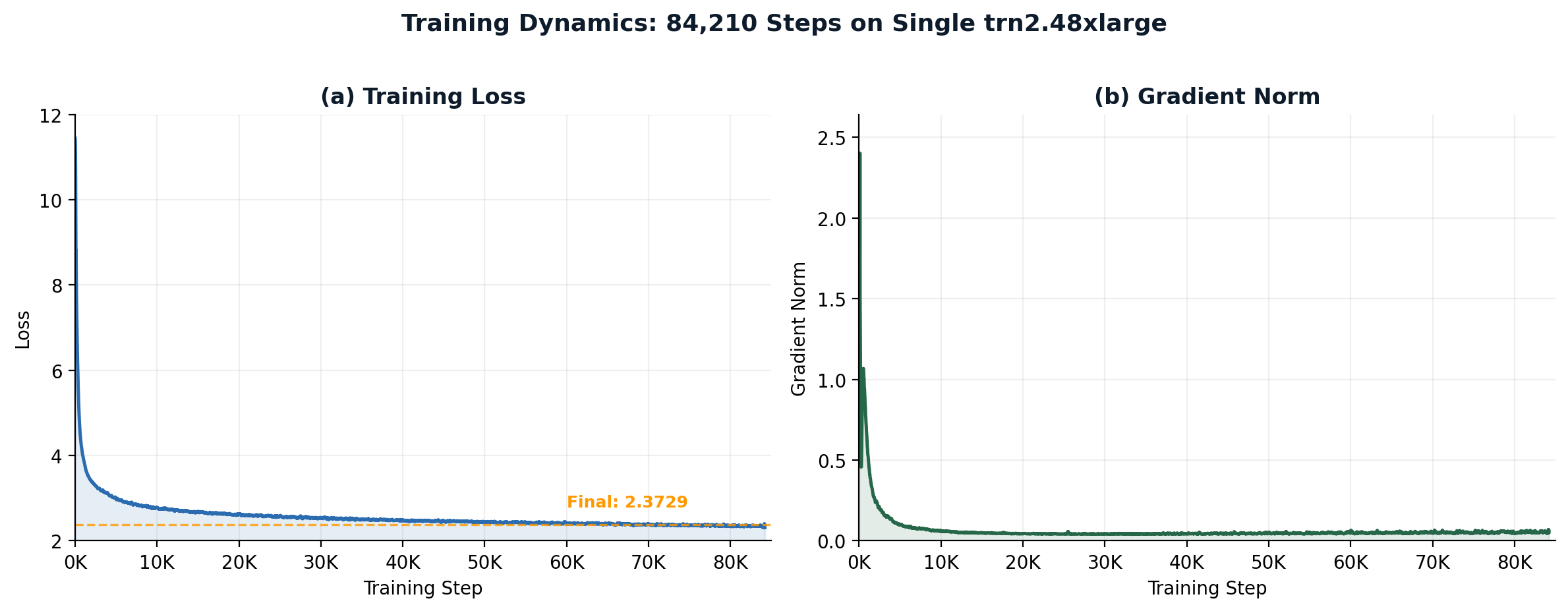
Determine 7: Coaching dynamics. (a) Loss 11.4 → 2.3729. (b) Gradient norm from TensorBoard knowledge.
Inference optimization on Trainium2
By an unmodified vLLM engine, the GenAIIC staff served 11,544 output tokens per second at 1,280 concurrent sequences on one trn2.48xlarge occasion.
Fixed serving state. The 29.5 MB recurrent state per sequence is roughly 82 instances smaller than a comparable KV cache at 8,192 tokens. Growing the immediate from 2,048 to eight,192 tokens added solely 0.5% to the fee per output token.
Unmodified vLLM. A wrapper replaces one attribute per decoder layer, the token mixer, to learn and write the recurrent state within the vLLM pool. As a result of the mannequin declares itself attention-free, vLLM allocates one fastened web page per sequence. Outputs matched the i14 reference token for token (48/48 steps on 3/3 prompts in BF16).
Discovering the bottleneck. A linear match of decode time in opposition to the variety of decoder layers L offers:

At L = 24, that’s 168.1 ms per step, 96.9 p.c of it contained in the decoder layers. The massive projections price 13.27 ms, close to the 12 ms HBM-streaming flooring. Most time went to small operators dispatched separately underneath keen PyTorch.
Scaling to a full occasion. With out tensor parallelism, throughput scales by means of replicas, with one engine and 20 sequences per logical NeuronCore. Keen throughput grew from 133 output tokens per second on one reproduction to six,772 on 64, the place host CPU utilization reached 82 p.c. Compiling the decode step eliminated per-operator dispatch and raised throughput 1.7 instances, to 11,544 (Determine 8).
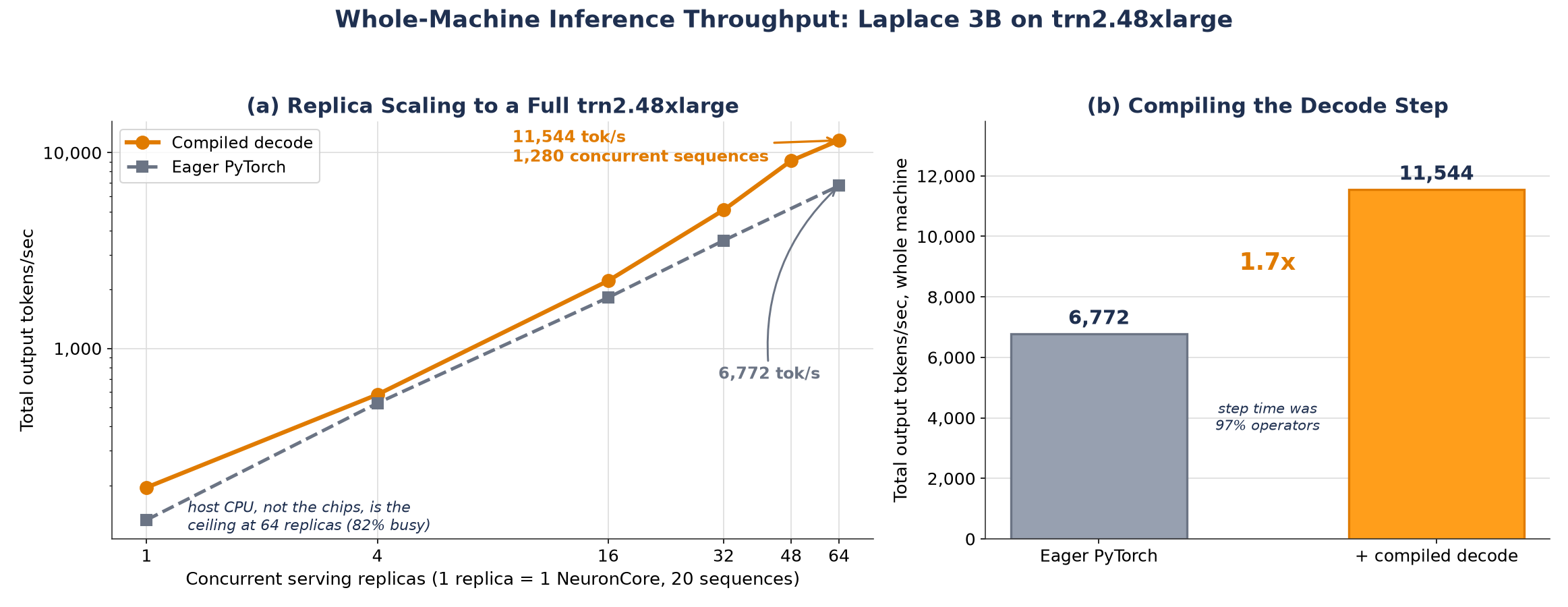
Determine 8: Entire-instance inference throughput. (a) Duplicate scaling on keen and compiled decode. (b) Compiled decode lifts throughput from 6,772 to 11,544 output tokens per second.
What fixed-batch benchmarks disguise. Underneath actual visitors, every new decode batch width is a individually compiled form whose first use prices about 11 seconds. These steps have been only one.1 p.c of the whole however consumed 47.5 p.c of decode time. Padding to fastened widths eliminated this price with bit-exact outcomes. Compiled decode then improved per-replica throughput 3.52 instances underneath staggered arrivals, in contrast with 1.46 instances on fastened batches. As a result of BF16 reassociation makes compiled output differ barely from keen, use keen decode when actual reproducibility issues.
Key takeaways
The undertaking produced classes throughout each coaching and inference:
- Native PyTorch can help customized architectures on Trainium2. i14 retained the GLA structure and used TorchNeuron Native for the ultimate implementation.
- Communication design issues for customized optimizers. The Muon all_to_all design lowered per-rank visitors by 24 instances and elevated coaching throughput by 1.63 instances.
- Fastened state retains inference reminiscence predictable. Every sequence makes use of 29.5 MB no matter context size.
- Profile earlier than compiling. Operator dispatch, quite than arithmetic or HBM bandwidth, accounted for many decode time.
- Benchmark life like arrival patterns. Fastened batches hid the price of compiling new shapes for altering batch widths.
Conclusion
Laplace 3B exhibits that AWS Trainium2 can help mannequin architectures past customary transformers. Utilizing native PyTorch by means of TorchNeuron Native and the AWS Neuron SDK, i14 skilled and served its GLA-based mannequin whereas preserving a hard and fast recurrent state.
For agentic methods, this adjustments a primary serving constraint. Longer histories don’t require a bigger per-sequence state, which will help groups retain extra context whereas preserving reminiscence use predictable.
If rising context is growing serving price, lowering concurrency, or limiting agent reminiscence, attempt i14 or contact your AWS account staff to judge Laplace 3B on AWS Trainium2.
Sources
Concerning the authors