Introduction
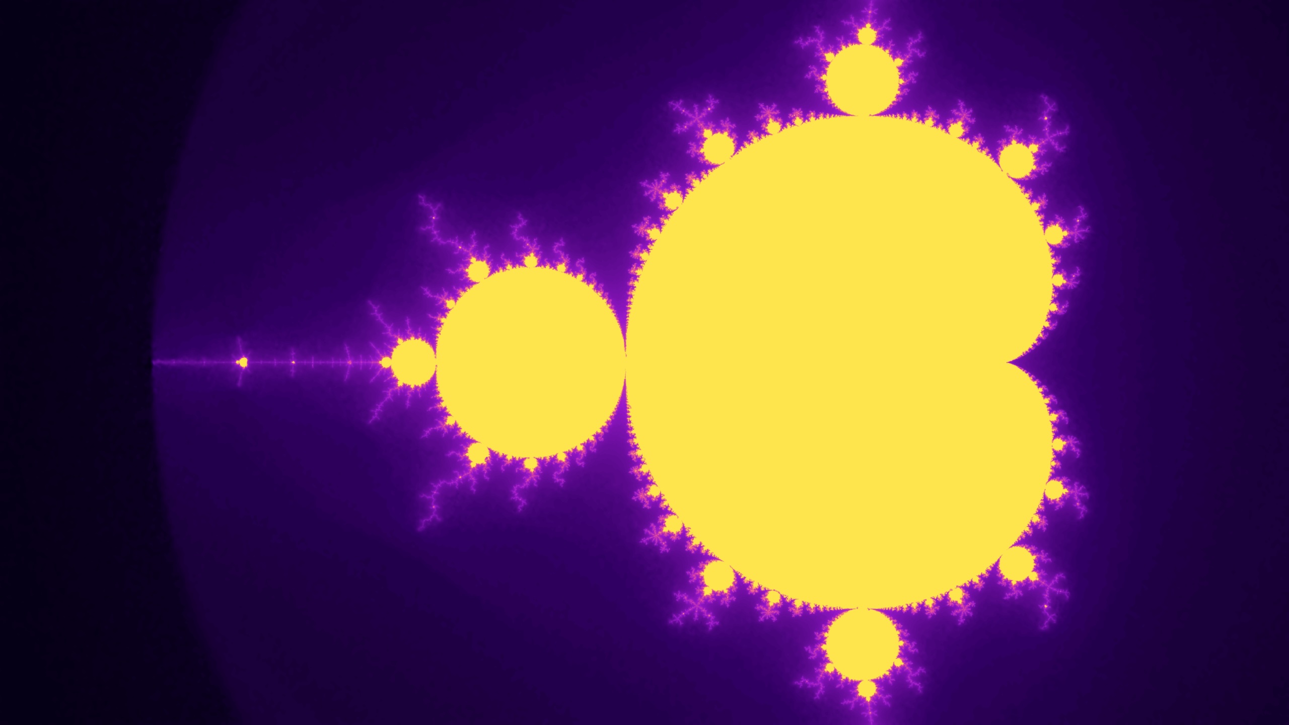
set is among the most stunning mathematical objects ever found, a fractal so intricate that regardless of how a lot you zoom in, you retain discovering infinite element. However what if we requested a neural community to study it?
At first look, this seems like an odd query. The Mandelbrot set is totally deterministic, there’s no knowledge, no noise, no hidden guidelines. However this simplicity makes it an ideal sandbox to review how neural networks symbolize complicated features.
On this article, we’ll discover how a easy neural community can study to approximate the Mandelbrot set, and the way Gaussian Fourier Options fully remodel its efficiency, turning blurry approximations into sharp fractal boundaries.
Alongside the way in which, we’ll dive into why vanilla multi-layer perceptrons (MLPs) wrestle with high-frequency patterns (the spectral bias drawback) and the way Fourier options remedy it.
The Mandelbrot Set
The Mandelbrot set is outlined over the complicated aircraft. For every complicated quantity (cin mathbb{C}), we take into account the iterative sequence:
$$z_{n+1} = z_n^2 + c, z_0 = 0$$
If this sequence stays bounded, then (c) belongs to the Mandelbrot set.
In follow, we approximate this situation utilizing the escape-time algorithm. The escape-time algorithm iterates the sequence as much as a hard and fast most variety of steps and displays the magnitude (|z_n|). If (|z_n|) exceeds a selected escape radius (usually 2), the sequence is assured to diverge, and (c) is assessed as exterior of the mandelbrot set. If the sequence doesn’t escape throughout the most variety of iterations, (c) is assumed to belong to the Mandelbrot set, with the iteration rely typically used for visualization functions.
Turning the Mandelbrot Set right into a Studying Drawback
To coach our neural community, we want two issues. First, we should outline a studying drawback, that’s, what the mannequin ought to predict and from what inputs. Second, we want labeled knowledge: a big assortment of input-output pairs drawn from that drawback.
Defining the Studying Drawback
At its core, the Mandelbrot set defines a perform over the complicated aircraft. Every level (c = x +iy in mathbb{C}) is mapped to an end result: both the sequence generated by the iteration stays bounded, or it diverges. This inmediately suggests a binary classification drawback, the place the enter is a fancy quantity and the output signifies whether or not the quantity is contained in the set or not.
Nevertheless, this formulation poses difficulties for studying. The boundary of the Mandelbrot set is infinitely complicated, and arbitrarily small perturbations in (c) can change the classification end result. From a studying perspective, this ends in a extremely discontinuous goal perform, making optimization unstable and data-inefficient.
To acquire a smoother and extra informative studying goal, we as an alternative reformulate the issue utilizing the escape-time data launched within the earlier part. Fairly than predicting a binary label, the mannequin is educated to foretell a steady variable derived from the iteration rely at which the sequence escapes.
To provide a steady goal perform we don’t use the uncooked escape iteration rely immediately. The uncooked escape iteration rely is a discrete amount, utilizing this could introduce discontinuities, notably close to the boundary of the Mandelbrot set, the place small modifications in (c) could cause massive jumps within the iteration rely. To handle this, we make use of a clean escape-time worth, which contains the escape iteration rely to supply a steady goal. As well as, we additionally apply a logarithmic scaling that spreads early escape values and compresses bigger ones, yielding a extra balanced goal distribution.
def smooth_escape(x: float, y: float, max_iter: int = 1000) -> float:
    c = complicated(x, y)
    z = 0j
    for n in vary(max_iter):
        z = z*z + c
        r2 = z.actual*z.actual + z.imag*z.imag
        if r2 > 4.0:
            r = math.sqrt(r2)
            mu = n + 1 - math.log(math.log(r)) / math.log(2.0)  # clean
            # log-scale to unfold small mu
            v = math.log1p(mu) / math.log1p(max_iter)
            return float(np.clip(v, 0.0, 1.0))
    return 1.0
With this definition, the Mandelbrot set turns into a regression drawback. The neural community is educated to approximate a perform $$f : mathbb{R}^2 rightarrow [0,1]$$
mapping spatial coordinates ((x, y)) within the complicated aircraft to a clean escape-time worth.
Knowledge Sampling Technique
A uniform sampling of the complicated aircraft can be extremely inefficient, most factors lie removed from the boundary and carry little data. To handle this, the dataset is biased in direction of boundary areas by oversampling and filtering factors whose escape values fall inside a predefined band.
def build_boundary_biased_dataset(
    n_total=800_000,
    frac_boundary=0.7,
    xlim=(-2.4, 1.0),
    res_for_ylim=(3840, 2160),
    ycenter=0.0,
    max_iter=1000,
    band=(0.35, 0.95),
    seed=0,
):
    """
    - Mixture of uniform samples + boundary-band samples.
    - 'band' selects factors with goal in (low, excessive), which tends to pay attention close to boundary.
    """
    rng = np.random.default_rng(seed)
    ylim = compute_ylim_from_x(xlim, res_for_ylim, ycenter=ycenter)

    n_boundary = int(n_total * frac_boundary)
    n_uniform  = n_total - n_boundary

    # Uniform set
    Xu = sample_uniform(n_uniform, xlim, ylim, seed=seed)

    # Boundary pool: oversample, then filter by band
    pool_factor = 20
    pool = sample_uniform(n_boundary * pool_factor, xlim, ylim, seed=seed + 1)

    yp = np.empty((pool.form[0],), dtype=np.float32)
    for i, (x, y) in enumerate(pool):
        yp[i] = smooth_escape(float(x), float(y), max_iter=max_iter)

    masks = (yp > band[0]) & (yp < band[1])
    Xb = pool[mask]
    yb = yp[mask]

    if len(Xb) < n_boundary:
        # If band too strict, loosen up it routinely
        hold = min(len(Xb), n_boundary)
        print(f"[warn] Boundary band too strict; received {len(Xb)} boundary factors, utilizing {hold}.")
        Xb = Xb[:keep]
        yb = yb[:keep]
        n_boundary = hold
        n_uniform = n_total - n_boundary
        Xu = sample_uniform(n_uniform, xlim, ylim, seed=seed)

    else:
        Xb = Xb[:n_boundary]
        yb = yb[:n_boundary]

    yu = np.empty((Xu.form[0],), dtype=np.float32)
    for i, (x, y) in enumerate(Xu):
        yu[i] = smooth_escape(float(x), float(y), max_iter=max_iter)

    X = np.concatenate([Xu, Xb], axis=0).astype(np.float32)
    y = np.concatenate([yu, yb], axis=0).astype(np.float32)

    # Shuffle as soon as
    perm = rng.permutation(X.form[0])
    return X[perm], y[perm], ylim
Baseline Mannequin: A Deep Residual MLP
Our first try makes use of a deep residual MLP that takes uncooked Cartesian coordinates ((x, y)) as enter and predicts the graceful escape worth.
# Baseline mannequin
class MLPRes(nn.Module):
    def __init__(
        self,
        hidden_dim=256,
        num_blocks=8,
        act="silu",
        dropout=0.0,
        out_dim=1,
    ):
        tremendous().__init__()
        activation = nn.ReLU if act.decrease() == "relu" else nn.SiLU

        self.in_proj = nn.Linear(2 , hidden_dim)
        self.in_act = activation()

        self.blocks = nn.Sequential(*[
            ResidualBlock(hidden_dim, act=act, dropout=dropout)
            for _ in range(num_blocks)
        ])

        self.out_ln = nn.LayerNorm(hidden_dim)
        self.out_act = activation()

        self.out_proj = nn.Linear(hidden_dim, out_dim)

    def ahead(self, x):
        x = self.in_proj(x)
        x = self.in_act(x)
        x = self.blocks(x)
        x = self.out_act(self.out_ln(x))
        return self.out_proj(x)
# Residual block
class ResidualBlock(nn.Module):
def __init__(self, dim: int, act: str = "silu", dropout: float = 0.0):
tremendous().__init__()
activation = nn.ReLU if act.decrease() == "relu" else nn.SiLU
# pre-norm-ish (LayerNorm helps quite a bit for stability with deep residual MLPs)
self.ln1 = nn.LayerNorm(dim)
self.fc1 = nn.Linear(dim, dim)
self.ln2 = nn.LayerNorm(dim)
self.fc2 = nn.Linear(dim, dim)
self.act = activation()
self.drop = nn.Dropout(dropout) if dropout and dropout > 0 else nn.Identification()
# elective: small init for the final layer to start out near-identity
nn.init.zeros_(self.fc2.weight)
nn.init.zeros_(self.fc2.bias)
def ahead(self, x):
h = self.ln1(x)
h = self.act(self.fc1(h))
h = self.drop(h)
h = self.ln2(h)
h = self.fc2(h)
return x + hThis community has ample capability: deep, residual, and educated on a big dataset with secure optimization.
Consequence

The worldwide form of the Mandelbrot set is clearly recognizable. Nevertheless, wonderful particulars close to the boundary are visibly blurred. Areas that ought to exhibit intricate fractal construction seem overly clean, and skinny filaments are both poorly outlined or completely lacking.
This isn’t a matter of decision, knowledge, or depth. So what goes mistaken?
The Spectral Bias Drawback
Neural networks have a well known drawback known as spectral bias:
they have a tendency to study low-frequency features first, and wrestle to symbolize features with fast oscillations or wonderful element.
The Mandelbrot boundary is dominated by extremely irregular, full of small-scale constructions, particularly close to its boundary. To seize it, the community would want to symbolize very high-frequency variations within the output as (x) and (y) change.
Fourier Options: Encoding Coordinates in Frequency Area
One of the crucial elegant options to the spectral bias drawback was launched in 2020 by Tancik et al. of their paper Fourier Options Let Networks Study Excessive Frequency Capabilities in Low Dimensional Domains.
The concept is to remodel the enter coordinates earlier than feeding them into the neural community. As an alternative of giving the uncooked ((x, y)), we cross their sinusoidal projection otno random instructions in a higher-dimensional area.
Formally:
$$gamma(x)=[sin(2 pi Bx),cos(2 pi Bx)]$$
the place (B in mathbb{R}^{d_{in}×d_{feat}}) is a random Gaussian matrix.
This mapping acts like a random Fourier foundation enlargement, letting the community extra simply symbolize high-frequency particulars.
class GaussianFourierFeatures(nn.Module):
    def __init__(self, in_dim=2, num_feats=256, sigma=5.0):
        tremendous().__init__()
        B = torch.randn(in_dim, num_feats) * sigma
        self.register_buffer("B", B)

    def ahead(self, x):
        proj = (2 * torch.pi) * (x @ self.B)
        return torch.cat([torch.sin(proj), torch.cos(proj)], dim=-1)
Multi-Scale Gaussian Fourier Options
A single frequency scale may not be ample. The Mandelbrot set reveals construction in any respect resolutions (a particular function of fractal geometry).
To seize this, we use multi-scale Gaussian Fourier options, combining a number of frequency bands:
class MultiScaleGaussianFourierFeatures(nn.Module):
    def __init__(self, in_dim=2, num_feats=512, sigmas=(2.0, 6.0, 10.0), seed=0):
        tremendous().__init__()
        # cut up options throughout scales
        okay = len(sigmas)
        per = [num_feats // k] * okay
        per[0] += num_feats - sum(per)

        Bs = []
        g = torch.Generator()
        g.manual_seed(seed)
        for s, m in zip(sigmas, per):
            B = torch.randn(in_dim, m, generator=g) * s
            Bs.append(B)

        self.register_buffer("B", torch.cat(Bs, dim=1))

    def ahead(self, x):
        proj = (2 * torch.pi) * (x @ self.B)
        return torch.cat([torch.sin(proj), torch.cos(proj)], dim=-1)
This successfully offers the community with a multi-resolution frequency foundation, completely aligned with the self-similar nature of fractals.
Closing Mannequin
The ultimate mannequin has the identical structure because the baseline mannequin, the one distinction is that it makes use of the MultiScaleGaussianFourierFeatures.
class MLPFourierRes(nn.Module):
    def __init__(
        self,
        num_feats=256,
        sigma=5.0,
        hidden_dim=256,
        num_blocks=8,
        act="silu",
        dropout=0.0,
        out_dim=1,
    ):
        tremendous().__init__()
        self.ff = MultiScaleGaussianFourierFeatures(
            2,
            num_feats=num_feats,
            sigmas=(2.0, 6.0, sigma),
            seed=0
        )

        self.in_proj = nn.Linear(2 * num_feats, hidden_dim)

        self.blocks = nn.Sequential(*[
            ResidualBlock(hidden_dim, act=act, dropout=dropout)
            for _ in range(num_blocks)
        ])

        self.out_ln = nn.LayerNorm(hidden_dim)
        activation = nn.ReLU if act.decrease() == "relu" else nn.SiLU
        self.out_act = activation()

        self.out_proj = nn.Linear(hidden_dim, out_dim)

    def ahead(self, x):
        x = self.ff(x)
        x = self.in_proj(x)
        x = self.blocks(x)
        x = self.out_act(self.out_ln(x))
        return self.out_proj(x)
Coaching Dynamics
Coaching With out Fourier Options
The mannequin slowly learns the general form of the Mandelbrot set, however then plateaus. Further coaching fails so as to add extra element.
Coaching With Fourier Options
Right here the coarse constructions seem first, adopted by progressively finer particulars. The mannequin continues to refine its prediction as an alternative of plateauing.
Closing Outcomes
Each fashions used the identical structure, dataset, and coaching process. The community is a deep residual multilayer perceptron (MLP) educated as a regression mannequin on the graceful escape-time formulation.
- Dataset: 1.000.000 samples from the complicated aircraft, with 70% of factors concentrated close to the fractal boundary because of the biased knowledge sampling.
- Structure: Residual MLP with 20 residual blocks, and a hidden dimension of 512 models.
- Activation Operate: SiLU
- Coaching: 100 epochs, batch dimension 4096, Adam-based optimizer, Cosine Annealing scheduler.
The one distinction between the 2 fashions is the illustration of the enter coordinates. The baseline mannequin makes use of the uncooked Cartesian coordinates, whereas the second mannequin makes use of the multi-scale Fourier Options for the illustration.
International View


Zoom 1 View


Zoom 2 View


Conclusions
Fractals such because the Mandelbrot set are an excessive instance of features dominated by high-frecuency constructions. Approximating them immediately from uncooked coordinates forces neural networks to synthesize more and more detailed oscillations, a process for which MLPs are poorly suited.
What this text exhibits is that the limitation isn’t architectural capability, knowledge quantity, or optimization. It’s illustration.
By encoding enter coordinates with multi-scale Gaussian Fourier Options, we shift a lot of the issue’s complexity into the enter area. Excessive-frequency construction turns into express, permitting an in any other case strange neural community to approximate a perform that might be too complicated in its unique type.
This concept extends past fractals. Coordinate-based neural networks are utilized in pc graphics, physics-informed studying, and singal processing. In all of those settings, the selection of enter encoding will be the distinction between clean approximations and wealthy, high-detailed construction.
Observe on visible property
All photographs, animations, and movies proven on this article had been generated by the writer from the outputs of the neural community fashions described above. No exterior fractal renderers or third-party visible property had been used. The complete code used for coaching, rendering photographs, and producing animations is accessible within the accompanying repository.


