NumPy for Absolute Inexperienced persons: A Mission-Based mostly Method to Information Evaluation

operating a sequence the place I construct mini tasks. I’ve constructed a Private Behavior and Climate Evaluation mission. However I haven’t actually gotten the possibility to discover the complete energy and functionality of NumPy. I need to attempt to perceive why NumPy is so helpful in knowledge evaluation. To wrap up this sequence, I’m going to be showcasing this in actual time.

I’ll be utilizing a fictional shopper or firm to make issues interactive. On this case, our shopper goes to be EnviroTech Dynamics, a worldwide operator of commercial sensor networks.

Presently, EnviroTech depends on outdated, loop-based Python scripts to course of over 1 million sensor readings each day. This course of is agonizingly gradual, delaying vital upkeep choices and impacting operational effectivity. They want a contemporary, high-performance resolution.

I’ve been tasked with making a NumPy-based proof-of-concept to reveal the best way to turbocharge their knowledge pipeline.

The Dataset: Simulated Sensor Readings

To show the idea, I’ll be working with a big, simulated dataset generated utilizing NumPy‘s random module, that includes entries with the next key arrays:

• Temperature —Every knowledge level represents how scorching a machine or system part is operating. These readings can rapidly assist us detect when a machine begins overheating — an indication of attainable failure, inefficiency, or security threat.
• Strain — knowledge displaying how a lot strain is increase contained in the system, and whether it is inside a protected vary
• Standing codes — characterize the well being or state of every machine or system at a given second. 0 (Regular), 1 (Warning), 2 (Vital), 3 (Defective/Lacking).

Mission Targets

The core aim is to supply 4 clear, vectorised options to EnviroTech’s knowledge challenges, demonstrating pace and energy. So I’ll be showcasing all of those:

• Efficiency and effectivity benchmark
• Foundational statistical baseline
• Vital anomaly detection and
• Information cleansing and imputation

By the top of this text, you must be capable to get a full grasp of NumPy and its usefulness in knowledge evaluation.

Goal 1: Efficiency and Effectivity Benchmark

First, we’d like an enormous dataset to make the pace distinction apparent. I’ll be utilizing the 1,000,000 temperature readings we deliberate earlier.

import numpy as np
# Set the dimensions of our knowledge
NUM_READINGS = 1_000_000

# Generate the Temperature array (1 million random floating-point numbers)
# We use a seed so the outcomes are the identical each time you run the code
np.random.seed(42)
mean_temp = 45.0
std_dev_temp = 12.0
temperature_data = np.random.regular(loc=mean_temp, scale=std_dev_temp, measurement=NUM_READINGS)

print(f”Information array measurement: {temperature_data.measurement} parts”)
print(f”First 5 temperatures: {temperature_data[:5]}”)

Output:

Information array measurement: 1000000 parts
First 5 temperatures: [50.96056984 43.34082839 52.77226246 63.27635828 42.1901595 ]

Now that we’ve our data. Let’s take a look at the effectiveness of NumPy.

Assuming we wished to calculate the common of all these parts utilizing a regular Python loop, it’ll go one thing like this.

# Operate utilizing a regular Python loop
def calculate_mean_loop(knowledge):
complete = 0
depend = 0
for worth in knowledge:
complete += worth
depend += 1
return complete / depend

# Let’s run it as soon as to ensure it really works
loop_mean = calculate_mean_loop(temperature_data)
print(f”Imply (Loop methodology): {loop_mean:.4f}”)

There’s nothing flawed with this methodology. However it’s fairly gradual, as a result of the pc has to course of every quantity one after the other, continuously transferring between the Python interpreter and the CPU.

To actually showcase the pace, I’ll be utilizing the%timeit command. This runs the code tons of of occasions to supply a dependable common execution time.

# Time the usual Python loop (will likely be gradual)
print(“ — — Timing the Python Loop — -”)
%timeit -n 10 -r 5 calculate_mean_loop(temperature_data)

Output

--- Timing the Python Loop ---
244 ms ± 51.5 ms per loop (imply ± std. dev. of 5 runs, 10 loops every)

Utilizing the -n 10, I’m mainly operating the code within the loop 10 occasions (to get a secure common), and utilizing the -r 5, the entire course of will likely be repeated 5 occasions (for much more stability).

Now, let’s evaluate this with NumPy vectorisation. And by vectorisation, it means your complete operation (common on this case) will likely be carried out on your complete array directly, utilizing extremely optimised C code within the background. 

Right here’s how the common will likely be calculated utilizing NumPy

# Utilizing the built-in NumPy imply perform
def calculate_mean_numpy(knowledge):
return np.imply(knowledge)
# Let’s run it as soon as to ensure it really works
numpy_mean = calculate_mean_numpy(temperature_data)
print(f”Imply (NumPy methodology): {numpy_mean:.4f}”)

Output:

Imply (NumPy methodology): 44.9808

Now let’s time it.

# Time the NumPy vectorized perform (will likely be quick)
print(“ — — Timing the NumPy Vectorization — -”)
%timeit -n 10 -r 5 calculate_mean_numpy(temperature_data)

Output:

--- Timing the NumPy Vectorization ---
1.49 ms ± 114 μs per loop (imply ± std. dev. of 5 runs, 10 loops every)

Now, that’s an enormous distinction. That’s like virtually non-existent. That’s the facility of vectorisation.

Let’s current this pace distinction to the shopper:

“We in contrast two strategies for performing the identical calculation on a million temperature readings — a conventional Python for-loop and a NumPy vectorized operation.

The distinction was dramatic: The pure Python loop took about 244 milliseconds per run whereas the NumPy model accomplished the identical process in simply 1.49 milliseconds.

That’s roughly a 160× pace enchancment.”

Goal 2: Foundational Statistical Baseline

One other cool function NumPy gives is the power to carry out fundamental to superior statistics — this fashion, you may get a great overview of what’s occurring in your dataset. It gives operations like:

• np.imply() — to calculate the common
• np.median — the center worth of the info
• np.std() — exhibits how unfold out your numbers are from the common
• np.percentile() — tells you the worth beneath which a sure share of your knowledge falls.

Now that we’ve managed to supply an alternate and environment friendly resolution to retrieve and carry out summaries and calculations on their large dataset, we will begin enjoying round with it.

We already managed to generate our simulated temperature knowledge. Let’s do the identical for strain. Calculating strain is a good way to reveal the power of NumPy to deal with a number of huge arrays very quickly in any respect.

For our shopper, it additionally permits me to showcase a well being test on their industrial methods.

Additionally, temperature and strain are sometimes associated. A sudden strain drop is likely to be the reason for a spike in temperature, or vice versa. Calculating baselines for each permits us to see if they’re drifting collectively or independently

# Generate the Strain array (Uniform distribution between 100.0 and 500.0)
np.random.seed(43) # Use a distinct seed for a brand new dataset
pressure_data = np.random.uniform(low=100.0, excessive=500.0, measurement=1_000_000)
print(“Information arrays prepared.”)

Output: 

Information arrays prepared.

Alright, let’s start our calculations.

print(“n — — Temperature Statistics — -”)
# 1. Imply and Median
temp_mean = np.imply(temperature_data)
temp_median = np.median(temperature_data)

# 2. Normal Deviation
temp_std = np.std(temperature_data)

# 3. Percentiles (Defining the 90% Regular Vary)
temp_p5 = np.percentile(temperature_data, 5) # fifth percentile
temp_p95 = np.percentile(temperature_data, 95) # ninety fifth percentile

# Formating our outcomes
print(f”Imply (Common): {temp_mean:.2f}°C”)
print(f”Median (Center): {temp_median:.2f}°C”)
print(f”Std. Deviation (Unfold): {temp_std:.2f}°C”)
print(f”90% Regular Vary: {temp_p5:.2f}°C to {temp_p95:.2f}°C”)

Right here’s the output:

--- Temperature Statistics ---
Imply (Common): 44.98°C
Median (Center): 44.99°C
Std. Deviation (Unfold): 12.00°C
90% Regular Vary: 25.24°C to 64.71°C

So to clarify what you’re seeing right here

The Imply (Common): 44.98°C mainly offers us a central level round which most readings are anticipated to fall. That is fairly cool as a result of we don’t must scan via your complete massive dataset. With this quantity, I’ve gotten a reasonably good thought of the place our temperature readings normally fall.

The Median (Center): 44.99°C is kind of equivalent to the imply should you discover. This tells us that there aren’t excessive outliers dragging the common too excessive or too low.

The usual deviation of 12°C means the temperatures fluctuate fairly a bit from the common. Principally, some days are a lot hotter or cooler than others. A decrease worth (say 3°C or 4°C) would have steered extra consistency, however 12°C signifies a extremely variable sample.

For the percentile, it mainly means most days hover between 25°C and 65°C,
If I had been to current this to the shopper, I may put it like this:

“On common, the system (or setting) maintains a temperature round 45°C, which serves as a dependable baseline for typical working or environmental circumstances. A deviation of 12°C signifies that temperature ranges fluctuate considerably across the common. 

To place it merely, the readings usually are not very secure. Lastly, 90% of all readings fall between 25°C and 65°C. This provides a sensible image of what “regular” appears to be like like, serving to you outline acceptable thresholds for alerts or upkeep. To enhance efficiency or reliability, we may determine the causes of excessive fluctuations (e.g., exterior warmth sources, air flow patterns, system load).”

Let’s calculate for strain additionally.

print(“n — — Strain Statistics — -”)
# Calculate all 5 measures for Strain
pressure_stats = {
“Imply”: np.imply(pressure_data),
“Median”: np.median(pressure_data),
“Std. Dev”: np.std(pressure_data),
“fifth %tile”: np.percentile(pressure_data, 5),
“ninety fifth %tile”: np.percentile(pressure_data, 95),
}
for label, worth in pressure_stats.objects():
print(f”{label:<12}: {worth:.2f} kPa”)

To enhance our codebase, I’m storing all of the calculations carried out in a dictionary known as strain stats, and I’m merely looping over the key-value pairs.

Right here’s the output:

--- Strain Statistics ---
Imply : 300.09 kPa
Median : 300.04 kPa
Std. Dev : 115.47 kPa
fifth %tile : 120.11 kPa
ninety fifth %tile : 480.09 kPa

If I had been to current this to the shopper. It’d go one thing like this:

“Our strain readings common round 300 kilopascals, and the median — the center worth — is nearly the identical. That tells us the strain distribution is kind of balanced total. Nonetheless, the normal deviation is about 115 kPa, which implies there’s loads of variation between readings. In different phrases, some readings are a lot larger or decrease than the standard 300 kPa degree.
Wanting on the percentiles, 90% of our readings fall between 120 and 480 kPa. That’s a variety, suggesting that strain circumstances usually are not secure — presumably fluctuating between high and low states throughout operation. So whereas the common appears to be like tremendous, the variability may level to inconsistent efficiency or environmental elements affecting the system.”

Goal 3: Vital Anomaly Identification

One in every of my favorite options of NumPy is the power to rapidly determine and filter out anomalies in your dataset. To reveal this, our fictional shopper, EnviroTech Dynamics, offered us with one other useful array that incorporates system standing codes. This tells us how the machine is constantly working. It’s merely a spread of codes (0–3).

• 0 → Regular
• 1 → Warning
• 2 → Vital
• 3 → Sensor Error

They obtain thousands and thousands of readings per day, and our job is to seek out each machine that’s each in a vital state and operating dangerously scorching.
Doing this manually, and even with a loop, would take ages. That is the place Boolean Indexing (masking) is available in. It lets us filter large datasets in milliseconds by making use of logical circumstances on to arrays, with out loops.

Earlier, we generated our temperature and strain knowledge. Let’s do the identical for the standing codes.

# Reusing 'temperature_data' from earlier
import numpy as np

np.random.seed(42) # For reproducibility

status_codes = np.random.selection(
a=[0, 1, 2, 3],
measurement=len(temperature_data),
p=[0.85, 0.10, 0.03, 0.02] # 0=Regular, 1=Warning, 2=Vital, 3=Offline
)

# Let’s preview our knowledge
print(status_codes[:5])

Output:

[0 2 0 0 0]

Every temperature studying now has an identical standing code. This permits us to pinpoint which sensors report issues and how extreme they’re.

Subsequent, we’ll want some kind of threshold or anomaly standards. In most situations, something above imply + 3 × normal deviation is taken into account a extreme outlier, the sort of studying you don’t need in your system. To compute that

temp_mean = np.imply(temperature_data)
temp_std = np.std(temperature_data)
SEVERITY_THRESHOLD = temp_mean + (3 * temp_std)
print(f”Extreme Outlier Threshold: {SEVERITY_THRESHOLD:.2f}°C”)

Output:

Extreme Outlier Threshold: 80.99°C

Subsequent, we’ll create two filters (masks) to isolate knowledge that meets our circumstances. One for readings the place the system standing is Vital (code 2) and one other for readings the place the temperature exceeds the brink.

# Masks 1 — Readings the place system standing = Vital (code 2)
critical_status_mask = (status_codes == 2)

# Masks 2 — Readings the place temperature exceeds threshold
high_temp_outlier_mask = (temperature_data > SEVERITY_THRESHOLD)

print(f”Vital standing readings: {critical_status_mask.sum()}”)
print(f”Excessive-temp outliers: {high_temp_outlier_mask.sum()}”)

Right here’s what’s occurring behind the scenes. NumPy creates two arrays stuffed with True or False. Each True marks a studying that satisfies the situation. True will likely be represented as 1, and False will likely be represented as 0. Summing them rapidly counts what number of match.

Right here’s the output:

Vital standing readings: 30178
Excessive-temp outliers: 1333

Let’s mix each anomalies earlier than printing our ultimate outcome. We wish readings which might be each vital and too scorching. NumPy permits us to filter on a number of circumstances utilizing logical operators. On this case, we’ll be utilizing the AND perform represented as &.

# Mix each circumstances with a logical AND
critical_anomaly_mask = critical_status_mask & high_temp_outlier_mask

# Extract precise temperatures of these anomalies
extracted_anomalies = temperature_data[critical_anomaly_mask]
anomaly_count = critical_anomaly_mask.sum()

print(“n — — Ultimate Outcomes — -”)
print(f”Complete Vital Anomalies: {anomaly_count}”)
print(f”Pattern Temperatures: {extracted_anomalies[:5]}”)

Output:

--- Ultimate Outcomes ---
Complete Vital Anomalies: 34
Pattern Temperatures: [81.9465697 81.11047892 82.23841531 86.65859372 81.146086 ]

Let’s current this to the shopper

“After analyzing a million temperature readings, our system detected 34 vital anomalies — readings that had been each flagged as ‘vital standing’ by the machine and exceeded the high-temperature threshold.

The primary few of those readings fall between 81°C and 86°C, which is nicely above our regular working vary of round 45°C. This means {that a} small variety of sensors are reporting harmful spikes, presumably indicating overheating or sensor malfunction.
In different phrases, whereas 99.99% of our knowledge appears to be like secure, these 34 factors characterize the actual spots the place we should always focus upkeep or examine additional.”

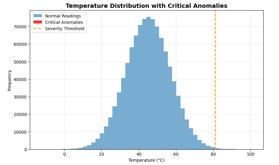
Let’s visualise this actual fast with matplotlib

Once I first plotted the outcomes, I anticipated to see a cluster of crimson bars displaying my vital anomalies. However there have been none.

At first, I assumed one thing was flawed, however then it clicked. Out of 1 million readings, solely 34 had been vital. That’s the fantastic thing about Boolean masking: it detects what your eyes can’t. Even when the anomalies conceal deep inside thousands and thousands of regular values, NumPy flags them in milliseconds.

Goal 4: Information Cleansing and Imputation

Lastly, NumPy lets you do away with inconsistencies and knowledge that doesn’t make sense. You might need come throughout the idea of information cleansing in knowledge evaluation. In Python, NumPy and Pandas are sometimes used to streamline this exercise. 

To reveal this, our status_codes include entries with a price of three (Defective/Lacking). If we use these defective temperature readings in our total evaluation, they may skew our outcomes. The answer is to interchange the defective readings with a statistically sound estimated worth.

Step one is to determine what worth we should always use to interchange the dangerous knowledge. The median is at all times a fantastic selection as a result of, not like the imply, it’s much less affected by excessive values.

# TASK: Determine the masks for ‘Legitimate’ knowledge (the place status_codes is NOT 3 — Defective/Lacking).
valid_data_mask = (status_codes != 3)

# TASK: Calculate the median temperature ONLY for the Legitimate knowledge factors. That is our imputation worth.
valid_median_temp = np.median(temperature_data[valid_data_mask])
print(f”Median of all legitimate readings: {valid_median_temp:.2f}°C”)

Output:

Median of all legitimate readings: 44.99°C

Now, we’ll carry out some conditional alternative utilizing the highly effective np.the place() perform. Right here’s a typical construction of the perform.

np.the place(Situation, Value_if_True, Value_if_False)

In our case:

• Situation: Is the standing code 3 (Defective/Lacking)?
• Worth if True: Use our calculated valid_median_temp.
• Worth if False: Preserve the unique temperature studying.

# TASK: Implement the conditional alternative utilizing np.the place().
cleaned_temperature_data = np.the place(
status_codes == 3, # CONDITION: Is the studying defective?
valid_median_temp, # VALUE_IF_TRUE: Substitute with the calculated median.
temperature_data # VALUE_IF_FALSE: Preserve the unique temperature worth.
)

# TASK: Print the whole variety of changed values.
imputed_count = (status_codes == 3).sum()
print(f”Complete Defective readings imputed: {imputed_count}”)

Output:

Complete Defective readings imputed: 20102

I didn’t count on the lacking values to be this a lot. It most likely affected our studying above not directly. Good factor, we managed to interchange them in seconds.

Now, let’s confirm the repair by checking the median for each the unique and cleaned knowledge

# TASK: Print the change within the total imply or median to indicate the affect of the cleansing.
print(f”nOriginal Median: {np.median(temperature_data):.2f}°C”)
print(f”Cleaned Median: {np.median(cleaned_temperature_data):.2f}°C”)

Output:

Unique Median: 44.99°C
Cleaned Median: 44.99°C

On this case, even after cleansing over 20,000 defective data, the median temperature remained regular at 44.99°C, indicating that the dataset is statistically sound and balanced.

Let’s current this to the shopper:

“Out of 1 million temperature readings, 20,102 had been marked as defective (standing code = 3). As an alternative of eradicating these defective data, we changed them with the median temperature worth (≈ 45°C) — a regular data-cleaning method that retains the dataset constant with out distorting the pattern.
Apparently, the median temperature remained unchanged (44.99°C) earlier than and after cleansing. That’s a great signal: it means the defective readings didn’t skew the dataset, and the alternative didn’t alter the general knowledge distribution.”

Conclusion

And there we go! We initiated this mission to handle a vital challenge for EnviroTech Dynamics: the necessity for sooner, loop-free knowledge evaluation. The facility of NumPy arrays and vectorisation allowed us to repair the issue and future-proof their analytical pipeline.

NumPy ndarray is the silent engine of your complete Python knowledge science ecosystem. Each main library, like Pandas, scikit-learn, TensorFlow, and PyTorch, makes use of NumPy arrays at its core for quick numerical computation.

By mastering NumPy, you’ve constructed a strong analytical basis. The following logical step for me is to maneuver from single arrays to structured evaluation with the Pandas library, which organises NumPy arrays into tables (DataFrames) for even simpler labelling and manipulation.

Thanks for studying! Be at liberty to attach with me:

LinkedIn

Twitter

YouTube