Introduction
Ever watched a badly dubbed film the place the lips don’t match the phrases? Or been on a video name the place somebody’s mouth strikes out of sync with their voice? These sync points are extra than simply annoying – they’re an actual downside in video manufacturing, broadcasting, and real-time communication. The Syncnet paper tackles this head-on with a intelligent self-supervised method that may routinely detect and repair audio-video sync issues with no need any guide annotations. What’s significantly cool is that the identical mannequin that fixes sync points also can work out who’s talking in a crowded room – all by studying the pure correlation between lip actions and speech sounds.
Core Purposes
The downstream duties which will be carried out with the output of the educated ConvNet have very important purposes which embody figuring out the lip-sync error in movies, detecting the speaker in a scene with a number of faces, and lip studying. Creating the lip-sync error utility, if the sync offset is current within the -1 to +1 second vary (this vary could possibly be different, however typically it suffices for TV broadcast audio-video) – that’s, video lags audio or vice-versa in -1 to +1 second – we are able to decide how a lot the offset is. For instance, say it comes out to be 200 ms audio lags video, which means video is 200 ms forward of audio, and in that case we are able to shift the audio 200 ms ahead and might make the offset sync problem close to 0 by this, so it additionally has purposes to make audio-video in sync (if offset lies within the vary we’ve taken right here -1 to +1 seconds).
Self-Supervised Coaching Method
The coaching methodology is self-supervised, which suggests no human annotations or guide labelling is required; the constructive and destructive pairs for coaching the mannequin occur with out guide labelling. This methodology assumes the info we get is already in sync (audio-video in sync), so we get the constructive pair already wherein the audio and video are in sync, and we make the false pair wherein audio and video aren’t in sync by shifting the audio by ± some seconds to make it async (false pair for coaching community). The benefit is that we are able to have virtually an infinite quantity of information to coach, offered it’s synced and already has no sync problem in supply, in order that constructive and destructive pairs will be made simply for coaching.
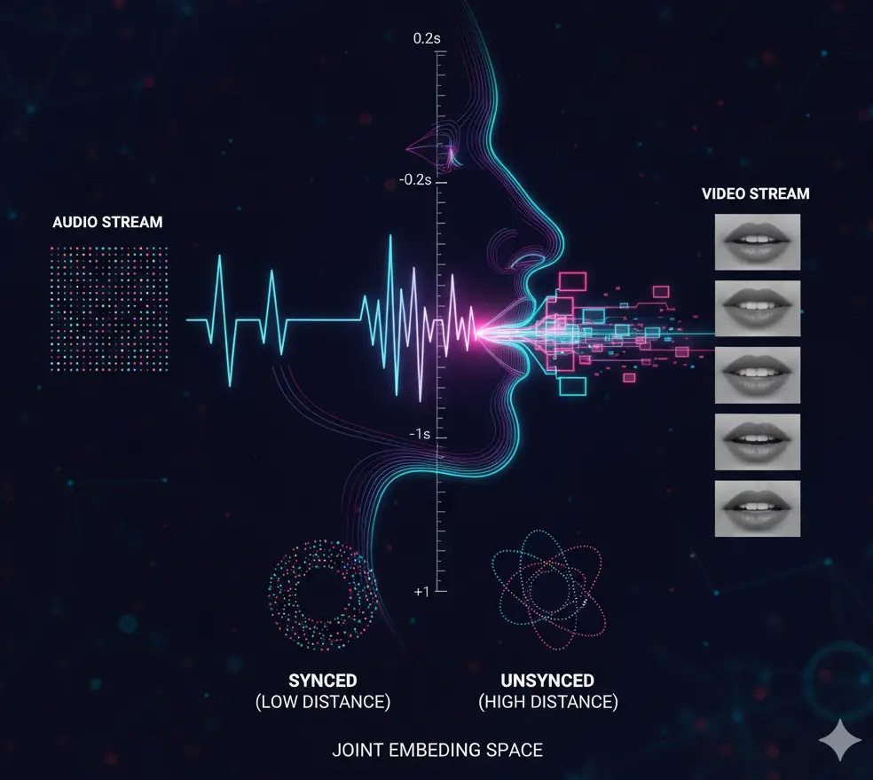
Community Structure: Twin-Stream CNN
Coming to the structure, it has 2 streams: audio stream and video stream, or in layman’s phrases, the structure is split into 2 branches – one for audio and one for video. Each streams count on 0.2 second enter. The audio stream expects 0.2 seconds of audio and the video stream expects 0.2 seconds of video. Each community architectures for audio and video streams are CNN-based, which count on 2D knowledge. For video (frames/pictures), CNN appears pure, however for audio, a CNN-based community can be educated. For each video and the corresponding audio, first their respective knowledge preprocessing is completed after which they’re fed into their respective CNN architectures.
Audio Information Preprocessing
Audio knowledge preprocessing – The uncooked 0.2 second audio goes via a sequence of steps to provide an MFCC 13 x 20 matrix. 13 are the DCT coefficients related for that audio chunk which symbolize the options for that audio, and 20 is within the time course, as a result of MFCC frequency was 100 Hz, so for 0.2 seconds, 20 samples will likely be there and every pattern’s DCT coefficients are represented by one column of the 13 x 20 matrix. The matrix 13 x 20 is enter to the CNN audio stream. Output of the community is a 256-dimensional embedding, illustration of the 0.2 second audio.
Video Information Preprocessing
Video preprocessing – The CNN right here expects enter of 111×111×5 (W×H×T), 5 frames of (h,w) = (111,111) gray-scale picture of mouth. Now for 25 fps, 0.2 seconds interprets to five frames. The uncooked video of 0.2 seconds goes via video preprocessing at 25 fps and will get transformed into 111x111x5 and fed into the CNN community. Output of the community is a 256-dimensional embedding, illustration of the 0.2 second video.
The audio preprocessing is less complicated and fewer complicated than video. Let’s perceive how the 0.2 second video and its corresponding audio are chosen from the unique supply. Our objective is to get a video clip the place there’s only one particular person and no scene change needs to be there within the 0.2 second, one one who’s talking within the 0.2 second period. Something aside from that is dangerous knowledge for our mannequin at this stage. So we run video knowledge preprocessing on the video, wherein we do scene detection, then face detection, after which face monitoring, crop the mouth half and convert all frames/pictures for the video into grayscale pictures of 111×111 and provides it to the CNN mannequin, and the corresponding audio half is transformed right into a 13×20 matrix and given to the audio CNN. The clips the place faces > 1 are rejected; there’s no scene change in 0.2 seconds clip as we’ve utilized scene detection within the pipeline. So what we’ve finally is a video wherein audio is there and one particular person is there in video, which suffices the first want of the info pipeline.
Joint Embedding Area Studying
The community learns a joint embedding area, which suggests the audio embedding and video embedding will likely be plotted in a typical embedding area. The joint embedding area could have these audio and video embeddings shut to one another that are in sync, and people audio and video embeddings will likely be far aside within the embedding area which aren’t in sync, that’s it. The Euclidean distance between synced audio and video embeddings will likely be much less and vice-versa.
Loss Operate and Coaching Refinement
The loss operate used is contrastive loss. For a constructive pair (sync audio-video 0.2 second instance), the sq. of Euclidean distance between audio and video embedding needs to be minimal; if that comes excessive, a penalty could be imposed, so for constructive pairs, the sq. of Euclidean distance is minimised, and for destructive pairs, max(margin – Euclidean distance, 0)² is minimised.
We refine the coaching knowledge by eradicating the false positives from our knowledge. Our knowledge nonetheless comprises false positives (noisy knowledge), and we take away the false positives by initially coaching the syncnet on noisy knowledge and eradicating these constructive pairs (that are marked as synced audio-video constructive pairs) which fail to move a sure threshold. The noisy knowledge (false positives) are there possibly due to dubbed video, another person talking over the speaker from behind, off-sync possibly current, or these kind of issues get filtered out on this refining step.
Inference and Purposes
Now the community will get educated, so let’s discuss inference and experimentation outcomes derived from the educated mannequin.
There’s check knowledge wherein constructive and destructive pairs for audio-video are current, so our mannequin’s inference ought to give low worth (min Euclidean distance) for constructive pairs within the check knowledge and excessive worth (max Euclidean distance) for destructive pairs within the check knowledge. That is one form of experiment or inference results of our mannequin.
Figuring out the offset can be one form of experiment, or we’d say one form of utility by our educated mannequin inference. The output could be the offset, like for instance audio leads by 200 ms or video leads by 170 ms – figuring out the sync offset worth for which video or audio lags. Meaning adjusting the offset decided by the mannequin ought to repair the sync problem and will make the clip in-sync from off-sync.
If adjusting the audio-video by the offset worth fixes the sync problem, which means success; in any other case failure of the mannequin (offered the synced audio to be current for that one mounted video within the vary we’re calculating the Euclidean distance between mounted video (0.2 s) and numerous audio chunks (0.2 s every, sliding over some -x to +x seconds vary, x = 1s)). This sync offset for the supply clip could possibly be both decided by calculating the sync offset worth for 1 single 0.2 second video from supply clip, or it could possibly be decided by doing a median over a number of 0.2 second samples from the supply clip after which give the averaged offset sync worth. The latter could be extra steady than the previous, additionally being proved by check knowledge benchmarks that taking common is the extra steady and higher option to inform the sync offset worth.
There’s a confidence rating related to this offset quantity which the mannequin offers, which is termed as AV sync confidence rating. For instance, it will be stated just like the supply clip has an offset, audio leads video by 300 ms with a confidence rating of 11. So understanding how this confidence rating is calculated is necessary, and let’s perceive it with an instance.
Sensible Instance: Offset and Confidence Rating Calculation
Let’s say we’ve a supply clip of 10 seconds and we all know this supply clip has sync offset wherein audio leads video by 300 ms. Now we’ll see how our syncnet is used to find out this offset.
We take ten 0.2 s movies as v1, v2, v3…….. v10.
Let’s perceive how sync rating and confidence rating will likely be calculated for v5, and comparable will occur with all 10 video bins/samples/chunks.
Supply Clip: 10 seconds whole
v1: 0.3-0.5s [–]
v2: 1.2-1.4s [–]
v3: 2.0-2.2s [–]
v4: 3.1-3.3s [–]
v5: 4.5-4.7s [–]
v6: 5.3-5.5s [–]
v7: 6.6-6.8s [–]
v8: 7.4-7.6s [–]
v9: 8.2-8.4s [–]
v10: 9.0-9.2s [–]
Let’s take v5 as one mounted video of 0.2s period. Now utilizing our educated syncnet mannequin, we’ll calculate the Euclidean distance between a number of audio chunks (will use a sliding window method) and this mounted video chunk. Right here’s how:
The audio sampling for v5 will occur from 3.5s to five.7s (±1s of v5), which supplies us a 2200ms (2.2 second) vary to look.
With overlapping home windows:
- Window dimension: 200ms (0.2s)
- Hop size: 100ms
- Variety of home windows: 21
Window 1: 3500-3700ms → Distance = 14.2
Window 2: 3600-3800ms → Distance = 13.8
Window 3: 3700-3900ms → Distance = 13.1
………………..
Window 8: 4200-4400ms → Distance = 2.8 ← MINIMUM (audio 300ms early)
Window 9: 4300-4500ms → Distance = 5.1
………………..
Window 20: 5400-5600ms → Distance = 14.5
Window 21: 5500-5700ms → Distance = 14.9
Sync offset for v5 = -300ms (audio leads video by 300ms) Confidence_v5 = median(~12.5) – min(2.8) = 9.7
So the arrogance rating for v5 for 300 ms offset is 9.7, and that is how confidence rating given by syncnet is calculated, which is the same as median(over all home windows or audio bins) – min(over all home windows or audio bins) for the mounted v5.
Equally, each different video bin has an offset worth with an related confidence rating.
v1 (0.3-0.5s): Offset = -290ms, Confidence = 8.5
v2 (1.2-1.4s): Offset = -315ms, Confidence = 9.2
v3 (2.0-2.2s): Offset = 0ms, Confidence = 0.8 (silence interval)
v4 (3.1-3.3s): Offset = -305ms, Confidence = 7.9
v5 (4.5-4.7s): Offset = -300ms, Confidence = 9.7
v6 (5.3-5.5s): Offset = -320ms, Confidence = 8.8
v7 (6.6-6.8s): Offset = -335ms, Confidence = 10.1
v8 (7.4-7.6s): Offset = -310ms, Confidence = 9.4
v9 (8.2-8.4s): Offset = -325ms, Confidence = 8.6
v10 (9.0-9.2s): Offset = -295ms, Confidence = 9.0
Averaging (ignoring low confidence v3): (-290 – 315 – 305 – 300 – 320 – 335 – 310 – 325 – 295) / 9 = -305ms
Or if together with all 10 with weighted averaging primarily based on confidence: Closing offset ≈ -300ms (audio leads video by 300ms) → That is how offset is calculated for the supply clip.
Vital notice – Both do weighted avg primarily based on confidence rating or take away those which have low confidence, as a result of not doing so will give:
Easy Common (INCLUDING silence) – WRONG: (-290 – 315 + 0 – 305 – 300 – 320 – 335 – 310 – 325 – 295) / 10 = -249.5ms That is approach off from the true 300ms!
This exhibits why the paper achieves 99% accuracy with averaging however solely 81% with single samples. Correct confidence-based filtering/weighting eliminates the deceptive silence samples.
Speaker Identification in Multi-Individual Scenes
Another necessary utility of sync rating is speaker identification in multi-person scenes. When a number of faces are seen however just one particular person’s audio is heard, syncnet computes the sync confidence for every face towards the identical audio stream. As an alternative of sliding audio temporally for one face, we consider all faces on the identical time level – every face’s mouth actions are in contrast with the present audio to generate confidence scores. The talking face naturally produces excessive confidence (sturdy audio-visual correlation) whereas silent faces yield low confidence (no correlation). By averaging these measurements over 10-100 frames, transient errors from blinks or movement blur get filtered out, just like how silence intervals had been dealt with in sync detection.
Conclusion
Syncnet demonstrates that typically the very best options come from rethinking the issue solely. As an alternative of requiring tedious guide labeling of sync errors, it cleverly makes use of the belief that almost all video content material begins out accurately synced – turning common movies into an infinite coaching dataset. The sweetness lies in its simplicity: prepare two CNNs to create embeddings the place synced audio-video pairs naturally cluster collectively. With 99% accuracy when averaging over a number of samples and the power to deal with all the things from broadcast TV to wild YouTube movies, this method has confirmed remarkably sturdy. Whether or not you’re fixing sync points in post-production or constructing the following video conferencing app, the rules behind Syncnet provide a sensible blueprint for fixing real-world audio-visual alignment issues at scale.


