A basic idea in Laptop Imaginative and prescient is knowing how pictures are saved and represented. On disk, picture recordsdata are encoded in numerous methods, from lossy, compressed JPEG recordsdata to lossless PNG recordsdata. When you load a picture right into a program and decode it from the respective file format, it’s going to almost certainly have an array-like construction that represents the pixels within the picture.
RGB
Every pixel comprises some coloration data about that particular level within the picture. Now the commonest option to signify this coloration is within the RGB house, the place every pixel has three values: purple, inexperienced and blue. These values describe how a lot of every coloration is current and they are going to be combined additively. So for instance, a picture with all values set to zero will likely be black. If all three values are set to 100%, the ensuing picture will likely be white.

Generally the order of those coloration channels might be swapped. One other frequent order is BGR, so the order is reversed. That is generally utilized in OpenCV and the default when studying or displaying pictures.
Alpha Channel
Photos may also include details about transparency. In that case, an extra alpha channel is current (RGBA). The alpha worth signifies the opacity of every pixel: an alpha of zero means the pixel is totally clear and a price of 100% represents a totally opaque pixel.

HSV
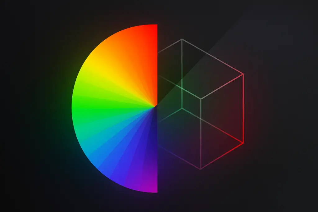
Now RGB(A) is just not the one option to signify colours. In truth there are various completely different coloration fashions that signify coloration. Probably the most helpful fashions is the HSV mannequin. On this mannequin, every coloration is represented by a hue, saturation and worth property. The hue describes the tone of coloration, regardless of brightness and saturation. Generally that is represented on a circle with values between 0 and 360 or 0 to 180, or just between 0 and 100%. Importantly, it’s cyclical, which means the values wrap round. The second property, the saturation describes how intense a coloration tone is, so a saturation of 0 ends in grey colours. Lastly the worth property describes the brightness of the colour, so a brightness of 0% is all the time black.

Now this coloration mannequin is extraordinarily useful in picture processing, because it permits us to decouple the colour tone from the saturation and brightness, which is inconceivable to do immediately in RGB. For instance, in order for you a transition between two colours and maintain the identical brightness through the full transition, this will likely be very complicated to attain utilizing the RGB coloration mannequin, whereas within the HSV mannequin that is simple by simply interpolating the hue.
Sensible Examples
We’ll take a look at three examples of learn how to work with these coloration areas in Python utilizing OpenCV. Within the first instance, we extract elements of a picture which can be of a sure coloration. Within the second half, we create a utility perform to transform colours between the colour areas. Lastly, within the third utility, we create a steady animation between two colours with fixed brightness and saturation.
1 – Colour Masks
The purpose of this half is to discover a masks that isolates colours primarily based on their hue in a picture. Within the following image, there are completely different coloured paper items that we need to separate.

Utilizing OpenCV, we are able to load the picture and convert it to the HSV coloration house. By default pictures are learn in BGR format, therefore we want the flag cv2.COLOR_BGR2HSV within the conversion:
Python">import cv2

img_bgr = cv2.imread("pictures/notes.png")
img_hsv = cv2.cvtColor(img_bgr, cv2.COLOR_BGR2HSV)
Now on the HSV picture we are able to apply a coloration filter utilizing the cv2.inRange perform to specify a decrease and higher sure for every property (hue, saturation, worth). With some experimentation I arrived on the following values for the filter:
| Property | Decrease Certain | Higher Certain |
|---|---|---|
| Hue | 90 | 110 |
| Saturation | 60 | 100 |
| Worth | 150 | 200 |
masks = cv2.inRange(
    src=img_hsv,
    lowerb=np.array([90, 60, 150]),
    upperb=np.array([110, 100, 200]),
)
The hue filter right here is constrained between 90 and 110, which corresponds to the sunshine blue paper on the backside of the picture. We additionally set a variety of the saturation and the brightness worth to get a fairly correct masks.

To indicate the outcomes, we first have to convert the single-channel masks again to a BGR picture form with 3 channels. Moreover, we are able to additionally apply the masks to the unique picture and visualize the outcome.
mask_bgr = cv2.cvtColor(masks, cv2.COLOR_GRAY2BGR)
img_bgr_masked = cv2.bitwise_and(img_bgr, img_bgr, masks=masks)

composite = cv2.hconcat([img_bgr, mask_bgr, img_bgr_masked])
cv2.imshow("Composite", composite)
By altering the hue vary, we are able to additionally isolate different items. For instance for the purple paper, we are able to specify the next vary:
| Property | Decrease Certain | Higher Certain |
|---|---|---|
| Hue | 160 | 175 |
| Saturation | 80 | 110 |
| Worth | 170 | 210 |

2 – Colour Conversion
Whereas OpenCV offers a useful perform to transform full pictures between coloration areas, it doesn’t present an out-of-the-box answer to transform single colours between coloration areas. We will write a easy wrapper that creates a small 1×1 pixel picture with an enter coloration, makes use of the built-in OpenCV perform to transform to a different coloration house and extract the colour of this single pixel once more.
def convert_color_space(enter: tuple[int, int, int], mode: int) -> tuple[int, int, int]:
    """
    Converts between coloration areas

    Args:
        enter: A tuple representing the colour in any coloration house (e.g., RGB or HSV).
        mode: The conversion mode (e.g., cv2.COLOR_RGB2HSV or cv2.COLOR_HSV2RGB).

    Returns:
        A tuple representing the colour within the goal coloration house.
    """
    px_img_hsv = np.array([[input]], dtype=np.uint8)
    px_img_bgr = cv2.cvtColor(px_img_hsv, mode)
    b, g, r = px_img_bgr[0][0]
    return int(b), int(g), int(r)
Now we are able to check the perform with any coloration. We will confirm that if we convert from RGB -> HSV -> RGB again to the unique format, we get the identical values.
red_rgb = (200, 120, 0)

red_hsv = convert_color_space(red_rgb, cv2.COLOR_RGB2HSV)
red_bgr = convert_color_space(red_rgb, cv2.COLOR_RGB2BGR)
red_rgb_back = convert_color_space(red_hsv, cv2.COLOR_HSV2RGB)

print(f"{red_rgb=}") # (200, 120, 0)
print(f"{red_hsv=}") # (18, 255, 200)
print(f"{red_bgr=}") # (0, 120, 200)
print(f"{red_rgb_back=}") # (200, 120, 0)
3 – Steady Colour Transition
On this third instance, we are going to create a transition between two colours with a relentless brightness and saturation interpolation. This will likely be in comparison with a direct interpolation between the preliminary and ultimate RGB values.
def interpolate_color_rgb(
    start_rgb: tuple[int, int, int], end_rgb: tuple[int, int, int], t: float
) -> tuple[int, int, int]:
    """
    Interpolates between two colours in RGB coloration house.
    Args:
        start_rgb: The beginning coloration in RGB format.
        end_rgb: The ending coloration in RGB format.
        t: A float between 0 and 1 representing the interpolation issue.
    Returns:
        The interpolated coloration in RGB format.
    """
    return (
        int(start_rgb[0] + (end_rgb[0] - start_rgb[0]) * t),
        int(start_rgb[1] + (end_rgb[1] - start_rgb[1]) * t),
        int(start_rgb[2] + (end_rgb[2] - start_rgb[2]) * t),
    )


def interpolate_color_hsv(
    start_rgb: tuple[int, int, int], end_rgb: tuple[int, int, int], t: float
) -> tuple[int, int, int]:
    """
    Interpolates between two colours in HSV coloration house.
    Args:
        start_rgb: The beginning coloration in RGB format.
        end_rgb: The ending coloration in RGB format.
        t: A float between 0 and 1 representing the interpolation issue.
    Returns:
        The interpolated coloration in RGB format.
    """
    start_hsv = convert_color_space(start_rgb, cv2.COLOR_RGB2HSV)
    end_hsv = convert_color_space(end_rgb, cv2.COLOR_RGB2HSV)

    hue = int(start_hsv[0] + (end_hsv[0] - start_hsv[0]) * t)
    saturation = int(start_hsv[1] + (end_hsv[1] - start_hsv[1]) * t)
    worth = int(start_hsv[2] + (end_hsv[2] - start_hsv[2]) * t)

    return convert_color_space((hue, saturation, worth), cv2.COLOR_HSV2RGB)
Now we are able to write a loop to match these two interpolation strategies. To create the picture, we use the np.full technique to fill all pixels of the picture array with a specified coloration. Utilizing cv2.hconcat we are able to mix the 2 pictures horizontally into one picture. Earlier than we show them, we have to convert to the OpenCV format BGR.
def run_transition_loop(
    color_start_rgb: tuple[int, int, int],
    color_end_rgb: tuple[int, int, int],
    fps: int,
    time_duration_secs: float,
    image_size: tuple[int, int],
) -> None:
    """
    Runs the colour transition loop.

    Args:
        color_start_rgb: The beginning coloration in RGB format.
        color_end_rgb: The ending coloration in RGB format.
        time_steps: The variety of time steps for the transition.
        time_duration_secs: The period of the transition in seconds.
        image_size: The scale of the pictures to be generated.
    """

    img_shape = (image_size[1], image_size[0], 3)
    num_steps = int(fps * time_duration_secs)

    for t in np.linspace(0, 1, num_steps):
        color_rgb_trans = interpolate_color_rgb(color_start_rgb, color_end_rgb, t)
        color_hue_trans = interpolate_color_hsv(color_start_rgb, color_end_rgb, t)

        img_rgb = np.full(form=img_shape, fill_value=color_rgb_trans, dtype=np.uint8)
        img_hsv = np.full(form=img_shape, fill_value=color_hue_trans, dtype=np.uint8)

        composite = cv2.hconcat((img_rgb, img_hsv))
        composite_bgr = cv2.cvtColor(composite, cv2.COLOR_RGB2BGR)

        cv2.imshow("Colour Transition", composite_bgr)

        key = cv2.waitKey(1000 // fps) & 0xFF
        if key == ord("q"):
            break

    cv2.destroyAllWindows()
Now we are able to merely name this perform with two colours for which we need to visualize the transition. Beneath I visualize the transition from blue to yellow.
run_transition_loop(
    color_start_rgb=(0, 0, 255),  # Blue
    color_end_rgb=(255, 255, 0),  # Yellow
    fps=25,
    time_duration_secs=5,
    image_size=(512, 256),
)
The distinction is kind of drastic. Whereas the saturation and brightness stay fixed in the suitable animation, they alter significantly for the transition that interpolates immediately within the RGB house.
For extra implementation particulars, take a look at the total supply code within the GitHub repository:
https://github.com/trflorian/auto-color-filter
All visualizations on this put up had been created by the writer.


